Level:
Correct: 0
Incorrect: 0
Marks: 0/0
Exam Practice
Course:
Topics:
Edexcel GCSE Statistics (Higher Paper 2) Smart practice A mixed round aimed at your weak spots
Unit 1
The statistical enquiry cycle
Statistical enquiry cycle stages 1 and 2; (a) Planning: 1a.01, 1a.02, 1a.03
Statistical enquiry cycle: planning and collecting
Statistical enquiry cycle stages 3, 4 and 5
Statistical enquiry cycle: interpreting and evaluating
Unit 2
The collection of data
(b) Types of data: 1b.01, 1b.02, 1b.03
Types of data and variables
(b) Types of data: 1b.04; (d) Collecting data: 1d.01, 1d.02
Primary and secondary data, reliability and validity
(c) Population and sampling: 1c.01, 1c.02, 1c.03
Populations, sampling frames and non-random sampling
(c) Population and sampling: 1c.04, 1c.05
Random and systematic sampling
(c) Population and sampling: 1c.06
Stratified sampling
(d) Collecting data: 1d.05, 1d.06
Problems with collected data and cleaning data
Unit 3
Processing, representing and analysing data
(a) Tabulation, diagrams and representation: 2a.01
Tabulation, tallies, pictograms and two-way tables
(a) Tabulation, diagrams and representation: 2a.01, 2a.02
Pie charts and comparative pie charts
(a) Tabulation, diagrams and representation: 2a.01
Stem and leaf diagrams
(a) Tabulation, diagrams and representation: 2a.02
Population pyramids, choropleth maps and 2D and 3D diagrams
(a) Tabulation, diagrams and representation: 2a.04
Histograms and frequency density
(a) Tabulation, diagrams and representation: 2a.05, 2a.06, 2a.07, 2a.08
Choosing representations and misleading diagrams
(a) Tabulation, diagrams and representation: 2a.09, 2a.10
Skewness
(b) Measures of central tendency: 2b.01, 2b.02, 2b.03
Mode, median and mean
(b) Measures of central tendency: 2b.01
Weighted mean and geometric mean
(c) Measures of dispersion: 2c.01, 2c.06
Standard deviation and standardised scores
(a) Tabulation, diagrams and representation: 2a.03; (c) Measures of dispersion: 2c.02, 2c.03
Box plots and outliers
(b) Measures of central tendency: 2b.03; (c) Measures of dispersion: 2c.04, 2c.05
Comparing distributions
(d) Further summary statistics: 2d.01
Index numbers
(d) Further summary statistics: 2d.02
Rates of change
(e) Scatter diagrams and correlation: 2e.01, 2e.02, 2e.03
Scatter diagrams, correlation and causation
(e) Scatter diagrams and correlation: 2e.04
Lines of best fit and regression lines
(e) Scatter diagrams and correlation: 2e.05, 2e.06, 2e.07, 2e.08
Spearman's rank and product moment correlation coefficients
(f) Time series: 2f.01, 2f.02; (b) 2b.01 mean seasonal variation
Time series, moving averages and seasonal variation
(g) Quality assurance: 2g.01, 2g.02
Quality assurance and control charts
(h) Estimation: 2h.01, 2h.02, 2h.03
Estimation, sample size and capture-recapture
Unit 4
Probability
3. Probability: 3p.01, 3p.02, 3p.03, 3p.04
Probability, expected frequency and risk
3. Probability: 3p.05, 3p.06, 3p.10
Experimental and theoretical probability and bias
3. Probability: 3p.11
Binomial distribution
3. Probability: 3p.12, 3p.13
Normal distribution
Avg
score:
–
Topics
done:
0/40

Skewness

Practise 15 exam-style questions on Skewness for Edexcel GCSE Statistics (Higher Paper 2). Write your answer as you would in the exam and get it marked in seconds against the mark scheme, point by point, with the Study Helper on hand if you get stuck.

  • 15 questions
  • 1–5 marks each
  • Instant marking
  • No sign-up needed
15 questions, marked as you go

Sample questions with model answers

Here are 4 of the questions in this topic, each with a model answer, an explanation of why it earns the marks and the mark scheme an examiner would use.

Question 1

1 mark

A farmer weighed the eggs laid by her hens in one week. The skew of the masses of the eggs is \(-0.4\)

Give an interpretation of this skew in the context of the masses of the eggs.

Model answer

The skew is negative, so the masses of the eggs below the median are more spread out than the masses above the median. Most eggs are fairly heavy, but a few are much lighter, which pulls the mean mass below the median mass.

Explanation

Negative skew means a longer tail of low values. Here a few small eggs stretch the lower half of the distribution, so the masses below the median are more spread out and the mean is less than the median. An interpretation must say what the skew means for the eggs, not just repeat 'negative skew'.

Mark scheme
  1. 1 mark

    B1 for a correct interpretation of negative skew in context, e.g.
    the masses below the median are more spread out than the masses above the median
    more than half of the eggs are heavier than the mean mass
    the mean mass of the eggs is less than the median mass
    most of the eggs are fairly heavy, with a few much lighter eggs

    oe. Must refer to the eggs or their masses. 'Negative skew' alone scores B0. B0 for 'more than half of the eggs are heavier than the median' (exactly half are), for any reference to the spread of the masses above or below the mean, and for 'most eggs are light' (an interpretation of positive skew).
Question 2

2 marks

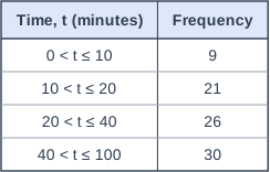
Ollie recorded the times, \(t\) minutes, that 86 shoppers spent in a shopping centre. The table shows his results.

Ollie says,
"The frequencies increase from each class to the next, so most shoppers spent a long time in the centre and the times have negative skew."

Explain why Ollie is wrong.

Table with columns "Time, t (minutes)", "Frequency". Time, t (minutes): 0 < t ≤ 10; Frequency: 9 | Time, t (minutes): 10 < t ≤ 20; Frequency: 21 | Time, t (minutes): 20 < t ≤ 40; Frequency: 26 | Time, t (minutes): 40 < t ≤ 100; Frequency: 30.

Model answer

The classes have different widths, so the frequencies cannot be compared directly. The frequency densities are \(9 \div 10 = 0.9\), \(21 \div 10 = 2.1\), \(26 \div 20 = 1.3\) and \(30 \div 60 = 0.5\). The times are most concentrated between 10 and 20 minutes, and the 30 shoppers in the last class are spread over 60 minutes.
The frequency densities rise to a peak at 10 to 20 minutes and then fall away, with a long tail of times up to 100 minutes, so the times have positive skew, not negative skew. Most shoppers (56 of the 86) spent 40 minutes or less in the centre.

Explanation

With unequal class widths, the shape of a distribution comes from the frequency densities, not the frequencies. A wide class can have a large frequency even though its values are thinly spread. Here the long tail is on the right, which is positive skew: the median (30 minutes) is much closer to the lower quartile (about 16 minutes) than to the upper quartile (57 minutes).

Mark scheme
  1. 1 mark

    B1 for the classes have different widths, so the frequencies cannot be compared directly: the frequency densities are 0.9, 2.1, 1.3 and 0.5, so the times are most concentrated in \(10 < t \le 20\) oe

    Must refer to the different class widths or to frequency density. Accept, for example, 'the last class has the most shoppers only because it is 60 minutes wide: its 30 shoppers are spread thinly'.

  2. 1 mark

    B1 for the times have positive skew, with a reason, e.g. the frequency densities rise to a peak at \(10 < t \le 20\) and then fall, with a long tail of times up to 100 minutes / the median (30 minutes) is much closer to the lower quartile (about 16 minutes) than to the upper quartile (57 minutes)

    Must state positive skew with a valid reason. Accept 'the estimated mean (37.7 minutes) is greater than the median (30 minutes)'. 'Positive skew' with no reason scores B0. This mark is independent of the first mark.

Question 3

3 marks

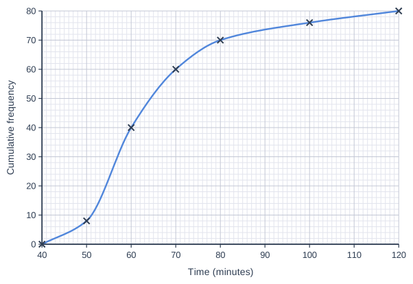
80 people took part in a 6 km charity walk. The cumulative frequency graph shows information about how long, \(t\) minutes, each walker took to finish.

Using the midpoints of the classes, estimates of the mean and the standard deviation of the times are
mean = 64.4 minutes   standard deviation = 15.5 minutes

skew \(= \dfrac{3(\text{mean} - \text{median})}{\text{standard deviation}}\)

Use the graph to find an estimate of the median time. Then calculate an estimate of the skew of the times. Give your answer correct to 2 decimal places.

Cumulative frequency graph on a grid of small squares. The horizontal axis is "Time (minutes)", from 40 to 120, numbered every 10, with 10 small squares between numbered values (each small square is 1). The vertical axis is "Cumulative frequency", from 0 to 80, numbered every 10, with 5 small squares between numbered values (each small square is 2). A smooth curve starts at (40, 0) and passes through (50, 8), (60, 40), (70, 60), (80, 70), (100, 76) and (120, 80) (each point is marked with a cross).

Model answer

Median: n/2 = 40. Reading across from 40 on the cumulative frequency axis to the graph, and down, gives a median of 60 minutes.
skew \(= \dfrac{3(64.4 - 60)}{15.5} = \dfrac{13.2}{15.5} = 0.851... = 0.85\)

Explanation

On a cumulative frequency graph the median is read at n/2 (here 40) on the vertical axis. The mean and standard deviation from the midpoints, and the median from the graph, are all estimates, so the skew is an estimate too. The skew is positive: a few walkers took much longer than the rest, which pulls the mean above the median.

Mark scheme
  1. 1 mark

    B1 for a median of 60 (minutes)

    Read at a cumulative frequency of 40 (n/2). Accept the reading at 40.5 ((n + 1)/2), 60.25. Accept readings from 59.5 to 60.5 inclusive. Answer-only rule for this question: A correct answer with no working scores B1M1A1.

  2. 1 mark

    M1 for \(\dfrac{3(64.4 - \text{their median})}{15.5}\), e.g. \(\dfrac{3(64.4 - 60)}{15.5}\)

    ft their median read from the graph. Using the midpoint of a class (e.g. 55) instead of a reading from the graph scores M0. \(\dfrac{3(\text{median} - \text{mean})}{15.5}\) scores M0.

  3. 1 mark

    A1 for 0.85

    awrt 0.85 (0.8516...) from a median of 60, or awrt 0.80 (0.8032...) from 60.25. Accept any answer from 0.75 to 0.95 inclusive that comes from a median in the accepted range (59.5 to 60.5). A correct answer with no working scores B1M1A1.

Question 4

4 marks

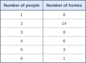
Jen surveyed the 40 homes in her street. The table shows the number of people living in each home.

standard deviation \(= \sqrt{\dfrac{\sum fx^2}{\sum f} - \left(\dfrac{\sum fx}{\sum f}\right)^2}\)
skew \(= \dfrac{3(\text{mean} - \text{median})}{\text{standard deviation}}\)

Calculate the skew of the numbers of people. Give your answer correct to 2 decimal places.

Table with columns "Number of people", "Number of homes". Number of people: 1; Number of homes: 8 | Number of people: 2; Number of homes: 14 | Number of people: 3; Number of homes: 8 | Number of people: 4; Number of homes: 6 | Number of people: 5; Number of homes: 3 | Number of people: 6; Number of homes: 1.

Model answer

Median: the 20th and 21st values. Cumulative frequencies: 8, 22, ..., so both are 2. Median = 2.
\(\sum fx = 8 + 28 + 24 + 24 + 15 + 6 = 105\), so mean \(= 105 \div 40 = 2.625\)
\(\sum fx^2 = 8 + 56 + 72 + 96 + 75 + 36 = 343\)
standard deviation \(= \sqrt{\dfrac{343}{40} - 2.625^2} = \sqrt{8.575 - 6.890625} = \sqrt{1.684375} = 1.2978...\)
skew \(= \dfrac{3(2.625 - 2)}{1.2978...} = 1.44\)

Explanation

From a frequency table, find the median by counting through the cumulative frequencies to the middle position, and the mean and standard deviation from \(\sum fx\) and \(\sum fx^2\). Remember that \(\sum fx^2\) means each value squared and then multiplied by its frequency. The positive skew comes from the few homes with 5 or 6 people.

Mark scheme
  1. 1 mark

    B1 for median = 2

    The 20th and 21st values (cumulative frequencies 8, 22, ...) are both 2. Accept the 20.5th value. A median of 3.5 (the middle of the values 1 to 6) scores B0. Answer-only rule for this question: A correct answer with no working scores full marks.

  2. 1 mark

    M1 for \(\sqrt{\dfrac{343}{40} - \left(\dfrac{105}{40}\right)^2}\) (= 1.2978...)

    \(\sum fx = 105\) (mean 2.625) and \(\sum fx^2 = 343\). Accept [1.29, 1.30] for the standard deviation. Using the \(n - 1\) divisor gives 1.314 and a skew of 1.43: this scores B1M1M1A0. Using \((\sum fx)^2\) in place of \(\sum fx^2\) scores M0.

  3. 1 mark

    M1 for \(\dfrac{3(2.625 - \text{their median})}{\text{their standard deviation}}\), e.g. \(\dfrac{3(2.625 - 2)}{1.2978}\)

    ft their median and standard deviation, which must be numerical. The mean must come from \(105 \div 40\).

  4. 1 mark

    A1 for 1.44

    awrt 1.44 (1.4447...). A standard deviation rounded to 1.3 also gives 1.44 (A1); a mean rounded to 2.6 gives 1.39 (A0). A correct answer with no working scores full marks.

Ready to try the rest? Every answer you write is marked against the mark scheme, so you can see exactly where the marks are.

Study Helper Hints first, answers after you try

Stuck on this one? Ask for a hint and I’ll point you in the right direction, without giving the answer away. Once you’ve checked your answer, I’ll show you how the marks are awarded.