
Level:
Correct: 0
Incorrect: 0
Marks: 0/0
Exam Practice
Course:
Topics:
Edexcel GCSE Statistics (Higher Paper 2) Smart practice A mixed round aimed at your weak spots
Unit 1
The statistical enquiry cycle
Statistical enquiry cycle stages 1 and 2; (a) Planning: 1a.01, 1a.02, 1a.03
Statistical enquiry cycle: planning and collecting
Statistical enquiry cycle stages 3, 4 and 5
Statistical enquiry cycle: interpreting and evaluating
Unit 2
The collection of data
(b) Types of data: 1b.01, 1b.02, 1b.03
Types of data and variables
(b) Types of data: 1b.04; (d) Collecting data: 1d.01, 1d.02
Primary and secondary data, reliability and validity
(c) Population and sampling: 1c.01, 1c.02, 1c.03
Populations, sampling frames and non-random sampling
(c) Population and sampling: 1c.04, 1c.05
Random and systematic sampling
(c) Population and sampling: 1c.06
Stratified sampling
(d) Collecting data: 1d.05, 1d.06
Problems with collected data and cleaning data
Unit 3
Processing, representing and analysing data
(a) Tabulation, diagrams and representation: 2a.01
Tabulation, tallies, pictograms and two-way tables
(a) Tabulation, diagrams and representation: 2a.01, 2a.02
Pie charts and comparative pie charts
(a) Tabulation, diagrams and representation: 2a.01
Stem and leaf diagrams
(a) Tabulation, diagrams and representation: 2a.02
Population pyramids, choropleth maps and 2D and 3D diagrams
(a) Tabulation, diagrams and representation: 2a.04
Histograms and frequency density
(a) Tabulation, diagrams and representation: 2a.05, 2a.06, 2a.07, 2a.08
Choosing representations and misleading diagrams
(a) Tabulation, diagrams and representation: 2a.09, 2a.10
Skewness
(b) Measures of central tendency: 2b.01, 2b.02, 2b.03
Mode, median and mean
(b) Measures of central tendency: 2b.01
Weighted mean and geometric mean
(c) Measures of dispersion: 2c.01, 2c.06
Standard deviation and standardised scores
(a) Tabulation, diagrams and representation: 2a.03; (c) Measures of dispersion: 2c.02, 2c.03
Box plots and outliers
(b) Measures of central tendency: 2b.03; (c) Measures of dispersion: 2c.04, 2c.05
Comparing distributions
(d) Further summary statistics: 2d.01
Index numbers
(d) Further summary statistics: 2d.02
Rates of change
(e) Scatter diagrams and correlation: 2e.01, 2e.02, 2e.03
Scatter diagrams, correlation and causation
(e) Scatter diagrams and correlation: 2e.04
Lines of best fit and regression lines
(e) Scatter diagrams and correlation: 2e.05, 2e.06, 2e.07, 2e.08
Spearman's rank and product moment correlation coefficients
(f) Time series: 2f.01, 2f.02; (b) 2b.01 mean seasonal variation
Time series, moving averages and seasonal variation
(g) Quality assurance: 2g.01, 2g.02
Quality assurance and control charts
(h) Estimation: 2h.01, 2h.02, 2h.03
Estimation, sample size and capture-recapture
Unit 4
Probability
3. Probability: 3p.01, 3p.02, 3p.03, 3p.04
Probability, expected frequency and risk
3. Probability: 3p.05, 3p.06, 3p.10
Experimental and theoretical probability and bias
3. Probability: 3p.11
Binomial distribution
3. Probability: 3p.12, 3p.13
Normal distribution
Avg
score:
–
Topics
done:
0/40

Normal distribution

Practise 17 exam-style questions on Normal distribution for Edexcel GCSE Statistics (Higher Paper 2). Write your answer as you would in the exam and get it marked in seconds against the mark scheme, point by point, with the Study Helper on hand if you get stuck.

  • 17 questions
  • 1–5 marks each
  • Instant marking
  • No sign-up needed
17 questions, marked as you go

Sample questions with model answers

Here are 4 of the questions in this topic, each with a model answer, an explanation of why it earns the marks and the mark scheme an examiner would use.

Question 1

1 mark

A bird ringer measured the wing lengths of 150 adult blackbirds. The histogram shows her results.

Give one feature of the histogram that suggests a normal distribution may be a suitable model for the wing lengths.
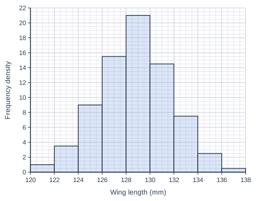
Histogram drawn on a grid of small squares. The horizontal axis is "Wing length (mm)", from 120 to 138, numbered every 2, with 4 small squares between numbered values (each small square is 0.5). The vertical axis is "Frequency density", from 0 to 22, numbered every 2, with 4 small squares between numbered values (each small square is 0.5). The bars touch, with no gaps between them. Bars: from 120 to 122, height 1; from 122 to 124, height 3.5; from 124 to 126, height 9; from 126 to 128, height 15.5; from 128 to 130, height 21; from 130 to 132, height 14.5; from 132 to 134, height 7.5; from 134 to 136, height 2.5; from 136 to 138, height 0.5.

Model answer

The histogram is roughly symmetrical and bell-shaped: it has one peak in the middle, at 128 to 130 mm, and the frequency densities fall away on both sides of it.

Explanation

A normal distribution is symmetrical and bell-shaped, with its mean, median and mode in the middle. A histogram with one central peak and tails that fall away evenly on both sides suggests a normal model may be suitable; a skewed or two-peaked histogram suggests it is not.

Mark scheme
  1. 1 mark

    B1 for e.g. it is (roughly) symmetrical / it is bell-shaped / it has a single peak in the middle (at 128 to 130 mm) and the frequency densities fall away evenly on both sides

    oe. B0 for 'wing length is continuous data' (true, but not a feature of the histogram). B0 for 'it has a peak' or 'it has a modal class' alone, with no reference to the middle or to symmetry. B0 for 'it is skewed'.
Question 2

2 marks

A farming co-operative records the daily milk yields of its 2000 cows. The daily milk yields, in litres, can be modelled by the normal distribution \(\text{N}(28, 16)\).

Estimate the number of cows with a daily milk yield between 16 litres and 20 litres.

Model answer

\(\sigma = \sqrt{16} = 4\)
16 litres \(= 28 - 3 \times 4\) and 20 litres \(= 28 - 2 \times 4\)
About 99.7% of the yields are within 3 s.d. of the mean and 95% within 2 s.d., so the percentage between 3 and 2 s.d. below the mean is \((99.7 - 95) \div 2 = 2.35\)%
Number of cows \(\approx 0.0235 \times 2000 = 47\)

Explanation

Turn the values into numbers of standard deviations from the mean first. The band between 2 and 3 standard deviations below the mean holds half of the difference between 'almost all' (about 99.7%) and 95%. Using 2.5% (treating 'almost all' as 100%) is also accepted.

Mark scheme
  1. 1 mark

    M1 for recognising that 16 and 20 are 3 and 2 standard deviations below the mean, and using \((99.7 - 95) \div 2\) (= 2.35%) oe

    Accept \((100 - 95) \div 2\) (= 2.5%, taking 'almost all' as 100%), \((99.8 - 95) \div 2\), or a calculator value (0.0214). Using 1 and 2 standard deviations (13.5%, giving 270 cows) or 5% (giving 100 cows) scores M0A0. Answer-only rule for this question: A correct answer with no working scores full marks.

  2. 1 mark

    A1 for an answer in the range 42.8 to 50 inclusive

    e.g. 47 (from 2.35%), 48 (from 2.4%), 50 (from 2.5%), 43 or 42.8 (from a calculator). A correct answer with no working scores full marks.

Question 3

3 marks

A factory uses two machines, A and B, to cut steel rods. A rod can be used only if its length is between 98 cm and 102 cm.

The lengths, in cm, of the rods cut by machine A can be modelled by \(\text{N}(100, 1)\).
The lengths, in cm, of the rods cut by machine B can be modelled by \(\text{N}(100.5, 0.25)\).

The manager says,
"Machine A is better, because the mean length of its rods is exactly 100 cm."

Is the manager correct? You must show your working.

Model answer

Machine A: \(\sigma = \sqrt{1} = 1\). 98 cm and 102 cm are \(100 \pm 2 \times 1\), 2 standard deviations from the mean, so about 95% of the rods can be used and about 5% cannot.
Machine B: \(\sigma = \sqrt{0.25} = 0.5\). Almost all rods are within 3 s.d. of the mean: \(100.5 \pm 3 \times 0.5\), from 99 cm to 102 cm, which is inside the limits.
So almost all of B's rods can be used, but about 5% of A's cannot. The manager is not correct: machine B is better, even though its mean is not exactly 100 cm.

Explanation

What matters is the proportion of rods inside the limits, which depends on the spread as well as the mean. B's small standard deviation keeps almost all of its rods within 3 standard deviations of 100.5 cm, which lies inside 98 to 102 cm. Remember that 1 and 0.25 are variances.

Mark scheme
  1. 1 mark

    B1 for machine A: 98 cm and 102 cm are 2 standard deviations from the mean (\(\sigma = 1\)), so about 5% of its rods cannot be used

    oe. Accept '95% of A's rods can be used'. Accept 4.6% from a calculator.

  2. 1 mark

    B1 for machine B: \(\sigma = \sqrt{0.25} = 0.5\), so 102 cm is 3 standard deviations above the mean (and 98 cm is 5 below), so almost all of its rods can be used

    oe. Accept 'almost all of B's rods are between 99 cm and 102 cm'. Using 0.25 as the standard deviation scores B0.

  3. 1 mark

    B1 for the manager is not correct: machine B is better because almost all of its rods can be used, compared with about 95% of A's (even though B's mean is not exactly 100 cm)

    Dependent on at least one of the previous marks. A decision with a reason based on the proportions of rods that can (or cannot) be used is needed. Answer only scores 0.

Question 4

4 marks

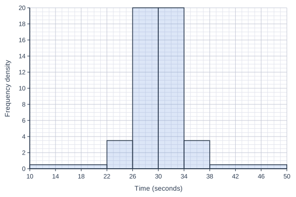
Each of 200 people was asked to say 'stop' when they thought 30 seconds had passed, without looking at a clock. The times, in seconds, are shown in the histogram.

The mean of the 200 times is 30.0 seconds and the standard deviation is 4.0 seconds.

Kian says,
"The histogram is symmetrical, so the times can be modelled by a normal distribution."

Use the histogram to assess Kian's claim. You must show your working.

Histogram drawn on a grid of small squares. The horizontal axis is "Time (seconds)", from 10 to 50, numbered every 4, with 4 small squares between numbered values (each small square is 1). The vertical axis is "Frequency density", from 0 to 20, numbered every 2, with 4 small squares between numbered values (each small square is 0.5). The bars touch, with no gaps between them. Bars: from 10 to 22, height 0.5; from 22 to 26, height 3.5; from 26 to 30, height 20; from 30 to 34, height 20; from 34 to 38, height 3.5; from 38 to 50, height 0.5.

Model answer

Within 1 s.d. of the mean: from 30.0 - 4.0 = 26 to 30.0 + 4.0 = 34 seconds.
Number of times \(= 4 \times 20 + 4 \times 20 = 160\), which is \(160 \div 200 = 80\)%
For a normal distribution about 68% of the times would be within 1 s.d. of the mean. 80% is much more than 68%: too many of the times are close to 30 seconds.
(Within 2 s.d., from 22 to 38 seconds: \(160 + 4 \times 3.5 + 4 \times 3.5 = 188\), which is 94%, close to 95%.)
So, although the histogram is symmetrical, Kian is not correct: a normal distribution is not a suitable model.

Explanation

Symmetry alone does not make a distribution normal. Check the proportions within 1 and 2 standard deviations against 68% and 95%: here 80% are within 1 standard deviation, so the distribution is too peaked in the middle. Remember that each frequency is the frequency density multiplied by the class width.

Mark scheme
  1. 1 mark

    M1 for using the histogram to find the number of times within 1 standard deviation of the mean (from 26 to 34 seconds), e.g. \(4 \times 20 + 4 \times 20\) (= 160)

    Frequency = frequency density \(\times\) class width. Also award M1 for a correct method for the number within 2 standard deviations (from 22 to 38 seconds), \(160 + 4 \times 3.5 + 4 \times 3.5\) (= 188), but the A1 is for the 1 standard deviation check only.

  2. 1 mark

    A1 for 80% (160 out of 200) within 1 standard deviation of the mean

    Accept 0.8.

  3. 1 mark

    B1 for comparing with the normal model: 80% is much more than the (about) 68% of a normal distribution that lie within 1 standard deviation of the mean

    ft their percentage from a correct method. The value 68% (or 'just over two thirds') must be stated. A check within 2 standard deviations may also be given: 188 (94%) is close to 95%, which does not change the conclusion; it is not needed for full marks. B0 for comparing 94% with 95% only.

  4. 1 mark

    B1 for Kian is not correct (a normal model is not suitable), because too many of the times are within 1 standard deviation of the mean, even though the histogram is symmetrical

    Dependent on the previous mark. A decision is needed. B0 for 'Kian is correct because the histogram is symmetrical and 94% is close to 95%'. Answer only scores 0.

Ready to try the rest? Every answer you write is marked against the mark scheme, so you can see exactly where the marks are.

Study Helper Hints first, answers after you try

Stuck on this one? Ask for a hint and I’ll point you in the right direction, without giving the answer away. Once you’ve checked your answer, I’ll show you how the marks are awarded.