
Level:
Correct: 0
Incorrect: 0
Marks: 0/0
Exam Practice
Course:
Topics:
Edexcel GCSE Statistics (Higher Paper 2) Smart practice A mixed round aimed at your weak spots
Unit 1
The statistical enquiry cycle
Statistical enquiry cycle stages 1 and 2; (a) Planning: 1a.01, 1a.02, 1a.03
Statistical enquiry cycle: planning and collecting
Statistical enquiry cycle stages 3, 4 and 5
Statistical enquiry cycle: interpreting and evaluating
Unit 2
The collection of data
(b) Types of data: 1b.01, 1b.02, 1b.03
Types of data and variables
(b) Types of data: 1b.04; (d) Collecting data: 1d.01, 1d.02
Primary and secondary data, reliability and validity
(c) Population and sampling: 1c.01, 1c.02, 1c.03
Populations, sampling frames and non-random sampling
(c) Population and sampling: 1c.04, 1c.05
Random and systematic sampling
(c) Population and sampling: 1c.06
Stratified sampling
(d) Collecting data: 1d.05, 1d.06
Problems with collected data and cleaning data
Unit 3
Processing, representing and analysing data
(a) Tabulation, diagrams and representation: 2a.01
Tabulation, tallies, pictograms and two-way tables
(a) Tabulation, diagrams and representation: 2a.01, 2a.02
Pie charts and comparative pie charts
(a) Tabulation, diagrams and representation: 2a.01
Stem and leaf diagrams
(a) Tabulation, diagrams and representation: 2a.02
Population pyramids, choropleth maps and 2D and 3D diagrams
(a) Tabulation, diagrams and representation: 2a.04
Histograms and frequency density
(a) Tabulation, diagrams and representation: 2a.05, 2a.06, 2a.07, 2a.08
Choosing representations and misleading diagrams
(a) Tabulation, diagrams and representation: 2a.09, 2a.10
Skewness
(b) Measures of central tendency: 2b.01, 2b.02, 2b.03
Mode, median and mean
(b) Measures of central tendency: 2b.01
Weighted mean and geometric mean
(c) Measures of dispersion: 2c.01, 2c.06
Standard deviation and standardised scores
(a) Tabulation, diagrams and representation: 2a.03; (c) Measures of dispersion: 2c.02, 2c.03
Box plots and outliers
(b) Measures of central tendency: 2b.03; (c) Measures of dispersion: 2c.04, 2c.05
Comparing distributions
(d) Further summary statistics: 2d.01
Index numbers
(d) Further summary statistics: 2d.02
Rates of change
(e) Scatter diagrams and correlation: 2e.01, 2e.02, 2e.03
Scatter diagrams, correlation and causation
(e) Scatter diagrams and correlation: 2e.04
Lines of best fit and regression lines
(e) Scatter diagrams and correlation: 2e.05, 2e.06, 2e.07, 2e.08
Spearman's rank and product moment correlation coefficients
(f) Time series: 2f.01, 2f.02; (b) 2b.01 mean seasonal variation
Time series, moving averages and seasonal variation
(g) Quality assurance: 2g.01, 2g.02
Quality assurance and control charts
(h) Estimation: 2h.01, 2h.02, 2h.03
Estimation, sample size and capture-recapture
Unit 4
Probability
3. Probability: 3p.01, 3p.02, 3p.03, 3p.04
Probability, expected frequency and risk
3. Probability: 3p.05, 3p.06, 3p.10
Experimental and theoretical probability and bias
3. Probability: 3p.11
Binomial distribution
3. Probability: 3p.12, 3p.13
Normal distribution
Avg
score:
–
Topics
done:
0/40

Scatter diagrams, correlation and causation

Practise 16 exam-style questions on Scatter diagrams, correlation and causation for Edexcel GCSE Statistics (Higher Paper 2). Write your answer as you would in the exam and get it marked in seconds against the mark scheme, point by point, with the Study Helper on hand if you get stuck.

  • 16 questions
  • 1–5 marks each
  • Instant marking
  • No sign-up needed
16 questions, marked as you go

Sample questions with model answers

Here are 4 of the questions in this topic, each with a model answer, an explanation of why it earns the marks and the mark scheme an examiner would use.

Question 1

1 mark

A librarian recorded the midday temperature, in °C, and the number of books borrowed on each of 14 days in October.

The scatter diagram shows her results.

Describe the correlation shown by the scatter diagram.
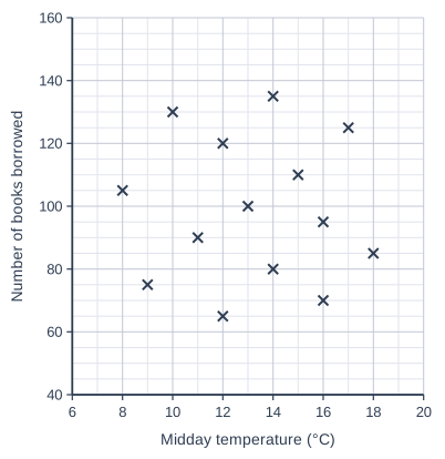
Scatter graph on a grid of small squares. The horizontal axis is "Midday temperature (°C)", from 6 to 20, numbered every 2, with 2 small squares between numbered values (each small square is 1). The vertical axis is "Number of books borrowed", from 40 to 160, numbered every 20, with 4 small squares between numbered values (each small square is 5). 14 points are plotted as crosses: (8, 105), (9, 75), (10, 130), (11, 90), (12, 65), (12, 120), (13, 100), (14, 80), (14, 135), (15, 110), (16, 70), (16, 95), (17, 125) and (18, 85).

Model answer

There is no correlation: the points are scattered with no pattern, so the number of books borrowed does not tend to rise or fall as the midday temperature increases.

Explanation

When the points show no upward or downward trend, there is no (zero) correlation: knowing the temperature tells you nothing about the number of books borrowed. Do not call it positive or negative because a few points seem to follow a direction, and avoid the word 'neutral'.

Mark scheme
  1. 1 mark

    B1 for no correlation

    Accept zero correlation / no relationship / no association between the temperature and the number of books borrowed. Condone 'very weak correlation' or 'almost no correlation', with or without a direction (e.g. 'very weak negative correlation'). Do not accept 'positive correlation', 'negative correlation', 'weak positive correlation' or 'weak negative correlation': the points show no upward or downward trend (r is about -0.02). Do not accept 'neutral'.
Question 2

2 marks

For 20 secondary schools in a county, there is strong positive correlation between the number of teachers who cycle to work and the number of students who achieved grade 9 in GCSE Mathematics last year.

A head teacher says,
"If more of our teachers cycle to work, more of our students will achieve grade 9."

Explain why the head teacher may be wrong.

Model answer

Correlation does not prove causation: getting more teachers to cycle would not make students achieve higher grades.

Both numbers are likely to be larger in bigger schools. A large school has more teachers, so more of them cycle to work, and more students, so more of them achieve grade 9. The correlation comes from the size of the schools.

Explanation

This is a spurious correlation: the two variables are correlated because both depend on a third variable, the size of the school. Comparing percentages instead (the percentage of teachers who cycle and the percentage of students achieving grade 9) would remove the effect of school size. An answer needs a statistical reason, not just 'that is silly'.

Mark scheme
  1. 1 mark

    B1 for correlation does not (necessarily) imply causation, e.g. the correlation does not show that teachers cycling causes more students to achieve grade 9

    Accept 'the correlation is spurious' or 'this is a coincidence, not a cause' oe. 'It doesn't make sense' with no statistical idea scores B0.

  2. 1 mark

    B1 for the size of the school affects both variables, e.g. larger schools have more teachers (so more teachers who cycle) and more students (so more students who achieve grade 9)

    Accept 'the number of students (or teachers) in each school' if it is linked to both variables. Condone 'it depends on the size of the school' with no further explanation. Accept another third variable only if it is clearly linked to both variables. 'Other factors affect grades', e.g. 'the quality of teaching', with no link to cycling, scores B0 for this mark.

Question 3

3 marks

Here is a list of words.

association   causation   extrapolation   interpolation   positive correlation   zero correlation

For each description, write down the word or phrase from the list that matches it.

Description 1: A change in one variable directly brings about a change in the other variable.
Description 2: Using a line of best fit to estimate a value outside the range of the data.
Description 3: Two variables are related in some way, but the relationship may not be linear.

Model answer

Description 1: causation
Description 2: extrapolation
Description 3: association

Explanation

Causation means that one variable causes changes in the other; correlation on its own does not show this. Extrapolation is estimating outside the range of the data (interpolation is within it). Association is any relationship between two variables, while correlation describes a linear relationship, where the points lie close to a straight line.

Mark scheme
  1. 1 mark

    B1 for Description 1: causation

    cao

  2. 1 mark

    B1 for Description 2: extrapolation

    Do not accept interpolation.

  3. 1 mark

    B1 for Description 3: association

    Do not accept positive correlation or zero correlation. If more than one word or phrase is given for a description, that description scores B0.

Question 4

4 marks

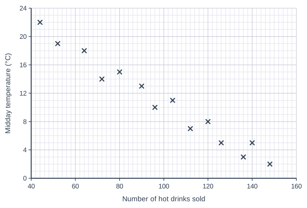
Sian recorded the midday temperature and the number of hot drinks sold at a park café on 14 days.

She drew the scatter diagram below.

Sian's teacher says that Sian has put the variables on the wrong axes.

Explain why the teacher is right.

Describe the strength and type of the correlation, and interpret it in context.

Scatter graph on a grid of small squares. The horizontal axis is "Number of hot drinks sold", from 40 to 160, numbered every 20, with 10 small squares between numbered values (each small square is 2). The vertical axis is "Midday temperature (°C)", from 0 to 24, numbered every 4, with 4 small squares between numbered values (each small square is 1). 14 points are plotted as crosses: (148, 2), (140, 5), (136, 3), (126, 5), (120, 8), (112, 7), (104, 11), (96, 10), (90, 13), (80, 15), (72, 14), (64, 18), (52, 19) and (44, 22).

Model answer

The number of hot drinks sold depends on the temperature (people buy more hot drinks on cold days), so the temperature is the explanatory variable and should be on the horizontal axis, with the number of hot drinks on the vertical axis.

The diagram shows strong negative correlation: on days with higher midday temperatures, fewer hot drinks were sold.

Explanation

By convention the dependent variable goes on the y-axis and the explanatory variable on the x-axis; swapping them does not change the correlation. The points lie close to a straight line sloping down, so the correlation is strong and negative. The interpretation must link the two variables: warmer days, fewer hot drinks.

Mark scheme
  1. 1 mark

    B1 for the temperature is the explanatory (independent) variable: the number of hot drinks sold depends on the temperature, so the number of hot drinks should be on the vertical axis (and the temperature on the horizontal axis)

    Accept 'the number of hot drinks is the dependent variable, so it should go on the y-axis' oe. Do not accept reasons based on the size of the numbers or the type of data.

  2. 1 mark

    B1 for strong

    Accept 'very strong'. Do not accept 'weak'.

  3. 1 mark

    B1 for negative

    Accept 'negative correlation' within a correct interpretation.

  4. 1 mark

    B1 for an interpretation in context, e.g. as the temperature increases, the number of hot drinks sold decreases / on warmer days fewer hot drinks were sold

    Accept the converse. Must refer to both the temperature and the number of hot drinks.

Ready to try the rest? Every answer you write is marked against the mark scheme, so you can see exactly where the marks are.

Study Helper Hints first, answers after you try

Stuck on this one? Ask for a hint and I’ll point you in the right direction, without giving the answer away. Once you’ve checked your answer, I’ll show you how the marks are awarded.