
Level:
Correct: 0
Incorrect: 0
Marks: 0/0
Exam Practice
Course:
Topics:
Edexcel GCSE Statistics (Higher Paper 2) Smart practice A mixed round aimed at your weak spots
Unit 1
The statistical enquiry cycle
Statistical enquiry cycle stages 1 and 2; (a) Planning: 1a.01, 1a.02, 1a.03
Statistical enquiry cycle: planning and collecting
Statistical enquiry cycle stages 3, 4 and 5
Statistical enquiry cycle: interpreting and evaluating
Unit 2
The collection of data
(b) Types of data: 1b.01, 1b.02, 1b.03
Types of data and variables
(b) Types of data: 1b.04; (d) Collecting data: 1d.01, 1d.02
Primary and secondary data, reliability and validity
(c) Population and sampling: 1c.01, 1c.02, 1c.03
Populations, sampling frames and non-random sampling
(c) Population and sampling: 1c.04, 1c.05
Random and systematic sampling
(c) Population and sampling: 1c.06
Stratified sampling
(d) Collecting data: 1d.05, 1d.06
Problems with collected data and cleaning data
Unit 3
Processing, representing and analysing data
(a) Tabulation, diagrams and representation: 2a.01
Tabulation, tallies, pictograms and two-way tables
(a) Tabulation, diagrams and representation: 2a.01, 2a.02
Pie charts and comparative pie charts
(a) Tabulation, diagrams and representation: 2a.01
Stem and leaf diagrams
(a) Tabulation, diagrams and representation: 2a.02
Population pyramids, choropleth maps and 2D and 3D diagrams
(a) Tabulation, diagrams and representation: 2a.04
Histograms and frequency density
(a) Tabulation, diagrams and representation: 2a.05, 2a.06, 2a.07, 2a.08
Choosing representations and misleading diagrams
(a) Tabulation, diagrams and representation: 2a.09, 2a.10
Skewness
(b) Measures of central tendency: 2b.01, 2b.02, 2b.03
Mode, median and mean
(b) Measures of central tendency: 2b.01
Weighted mean and geometric mean
(c) Measures of dispersion: 2c.01, 2c.06
Standard deviation and standardised scores
(a) Tabulation, diagrams and representation: 2a.03; (c) Measures of dispersion: 2c.02, 2c.03
Box plots and outliers
(b) Measures of central tendency: 2b.03; (c) Measures of dispersion: 2c.04, 2c.05
Comparing distributions
(d) Further summary statistics: 2d.01
Index numbers
(d) Further summary statistics: 2d.02
Rates of change
(e) Scatter diagrams and correlation: 2e.01, 2e.02, 2e.03
Scatter diagrams, correlation and causation
(e) Scatter diagrams and correlation: 2e.04
Lines of best fit and regression lines
(e) Scatter diagrams and correlation: 2e.05, 2e.06, 2e.07, 2e.08
Spearman's rank and product moment correlation coefficients
(f) Time series: 2f.01, 2f.02; (b) 2b.01 mean seasonal variation
Time series, moving averages and seasonal variation
(g) Quality assurance: 2g.01, 2g.02
Quality assurance and control charts
(h) Estimation: 2h.01, 2h.02, 2h.03
Estimation, sample size and capture-recapture
Unit 4
Probability
3. Probability: 3p.01, 3p.02, 3p.03, 3p.04
Probability, expected frequency and risk
3. Probability: 3p.05, 3p.06, 3p.10
Experimental and theoretical probability and bias
3. Probability: 3p.11
Binomial distribution
3. Probability: 3p.12, 3p.13
Normal distribution
Avg
score:
–
Topics
done:
0/40

Lines of best fit and regression lines

Practise 17 exam-style questions on Lines of best fit and regression lines for Edexcel GCSE Statistics (Higher Paper 2). Write your answer as you would in the exam and get it marked in seconds against the mark scheme, point by point, with the Study Helper on hand if you get stuck.

  • 17 questions
  • 1–5 marks each
  • Instant marking
  • No sign-up needed
17 questions, marked as you go

Sample questions with model answers

Here are 4 of the questions in this topic, each with a model answer, an explanation of why it earns the marks and the mark scheme an examiner would use.

Question 1

1 mark

A taxi firm recorded the length, \(x\) miles, and the fare, \(y\) pounds, for 50 journeys. The journeys were between 0.5 miles and 15 miles long.

The equation of the regression line is
\(y = 3.2 + 2.15x\)

Interpret the value 3.2 in this context.

Model answer

3.2 is the estimated fare, £3.20, for a journey of 0 miles: it is like a fixed starting charge that is paid on every journey before the cost of the distance is added.

Explanation

The intercept a is the value of y when x = 0. Interpret it only when x = 0 makes sense in context; a journey of almost 0 miles is possible, so £3.20 can be read as the fixed part of the fare. Do not confuse the intercept with the gradient, which is £2.15 per mile.

Mark scheme
  1. 1 mark

    B1 for e.g. the estimated fare for a journey of 0 miles is £3.20 / the fixed (starting) charge for a journey is about £3.20

    Must refer to £3.20 (or 3.2 pounds) and to a distance of 0 miles or the start of the journey. Accept '£3.20 is the fare before any distance is travelled' oe. Do not accept 'the fare increases by £3.20 per mile' (that confuses the intercept with the gradient). An answer that says 3.2 should not be interpreted because 0 miles is outside the data scores B0: a journey of almost 0 miles is realistic, so the intercept has a sensible meaning here. An interpretation followed by a caution, e.g. '... but 0 miles is just outside the range of the data', still scores B1.
Question 2

2 marks

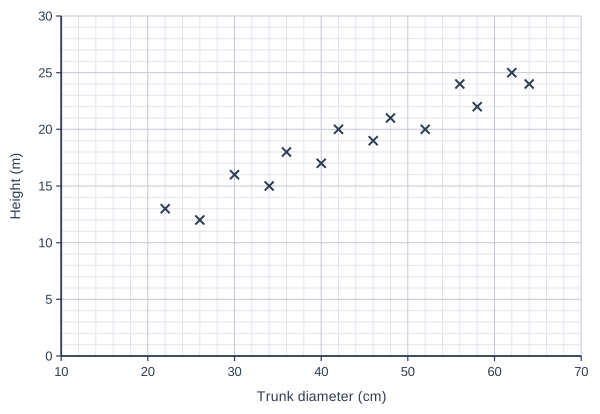
A tree surgeon measured the trunk diameter, in cm, and the height, in metres, of 14 oak trees in a park.

The scatter diagram shows this information.

The double mean point of the data is (44, 19).

Using a line of best fit that passes through the double mean point, estimate the height of an oak tree in the park with a trunk diameter of 60 cm.

Scatter graph on a grid of small squares. The horizontal axis is "Trunk diameter (cm)", from 10 to 70, numbered every 10, with 5 small squares between numbered values (each small square is 2). The vertical axis is "Height (m)", from 0 to 30, numbered every 5, with 5 small squares between numbered values (each small square is 1). 14 points are plotted as crosses: (22, 13), (26, 12), (30, 16), (34, 15), (36, 18), (40, 17), (42, 20), (46, 19), (48, 21), (52, 20), (56, 24), (58, 22), (62, 25) and (64, 24).

Model answer

A line of best fit through the double mean point (44, 19) that follows the points also passes close to (64, 25), so its gradient is about \(\dfrac{25 - 19}{64 - 44} = 0.3\).

At 60 cm: \(19 + 0.3 \times (60 - 44) = 19 + 4.8 = 23.8\)

The estimated height is about 23.8 m.

Explanation

A line of best fit should pass through the double mean point and follow the trend of the points, with the points balanced on either side. Then read up from 60 cm to the line and across to the height axis. This is an interpolation (60 cm is within the range of the diameters, 22 cm to 64 cm), so the estimate should be reasonably reliable.

Mark scheme
  1. 1 mark

    M1 for a line of best fit through (44, 19) used to find the height at 60 cm, e.g. a gradient of about 0.3 giving \(19 + 0.3 \times 16\)

    Implied by an answer in the range 23 to 24.5. A line that does not pass through (44, 19), or an estimate from the nearest plotted points only (e.g. 25 from the tree at (62, 25)), scores M0. Answer-only rule for this question: A correct answer with no working scores M1 A1.

  2. 1 mark

    A1 for an answer in the range 23 to 24.5 (m)

    A line through (44, 19) that follows the points has a gradient between about 0.29 and 0.32, giving 23.7 m to 24.1 m at 60 cm; the range allows a little more for lines drawn by eye. A correct answer with no working scores M1 A1.

Question 3

3 marks

For each team in a hockey league over several seasons, a statistician recorded the number of points, \(x\), that the team scored in the first half of a season and the number of points, \(y\), that it scored in the second half of the same season. She has 60 pairs of values, with \(x\) between 5 and 45.

The equation of the regression line is
\(y = 6 + 0.8x\)

Interpret the gradient of the regression line in this context.

Emma says,
"The regression line predicts that a team that scored more than 30 points in the first half of a season will score fewer points in the second half."

Show that Emma is correct.

Model answer

Gradient: for every extra point a team scores in the first half of the season, the predicted number of points in the second half increases by 0.8.

The prediction is fewer points in the second half when
\(6 + 0.8x < x\)
\(6 < 0.2x\)
\(x > 30\)

So for any team that scored more than 30 points in the first half, the regression line predicts fewer points in the second half: Emma is correct.

Explanation

The predicted second-half score equals the first-half score where 6 + 0.8x = x, which is at x = 30. Because the gradient 0.8 is less than 1, the line rises more slowly than y = x, so for x above 30 the prediction is lower than x. One numerical example is not enough to show that the statement is true for every value above 30.

Mark scheme
  1. 1 mark

    B1 for e.g. for every extra point scored in the first half of the season, the estimated number of points scored in the second half increases by 0.8

    Must refer to 0.8 points and to one extra point in the first half. Do not credit the converse.

  2. 1 mark

    M1 for forming \(6 + 0.8x < x\) (or \(6 + 0.8x = x\), or \(0.2x > 6\)) oe, or for showing that the line gives 30 when \(x = 30\) and that the gradient is less than 1

    A check for one value only, e.g. \(6 + 0.8 \times 40 = 38 < 40\), scores M1 A0.

  3. 1 mark

    A1 for showing \(x > 30\) (from \(0.2x > 6\)) with the conclusion that, for every value of \(x\) above 30, the predicted second-half points are fewer than the first-half points

    This is a show question: the full method must be seen. Accept the argument 'the line gives y = x at x = 30, and as the gradient 0.8 is less than 1, y increases more slowly than x, so y < x for x > 30'.

Question 4

4 marks

A small business compared two courier firms. For parcels sent a distance of \(x\) km, it recorded the delivery time, \(y\) hours. For both firms, the distances were between 20 km and 400 km.

The equations of the regression lines are
Firm P: \(y = 4.5 + 0.06x\)
Firm Q: \(y = 9 + 0.035x\)

The business wants to use the firm with the shorter estimated delivery time for each parcel.

Explain how the business could use the regression lines to decide which firm to use for each parcel. You must show your working.

Model answer

Where both firms have the same estimated delivery time:
\(4.5 + 0.06x = 9 + 0.035x\)
\(0.025x = 4.5\)
\(x = 180\)

At 180 km both firms have an estimated delivery time of \(4.5 + 0.06 \times 180 = 15.3\) hours.

Firm P has the smaller intercept but the larger gradient. For example, at 100 km Firm P takes an estimated 10.5 hours and Firm Q 12.5 hours. So the business should use Firm P for parcels going less than 180 km and Firm Q for parcels going more than 180 km.

Explanation

Two regression lines give the same estimate where they intersect, so solve the two equations together. On one side of the intersection one line is lower and on the other side the other line is lower; check with a value such as 100 km. The decision applies within the range of the data (20 km to 400 km).

Mark scheme
  1. 1 mark

    M1 for equating the two equations, e.g. \(4.5 + 0.06x = 9 + 0.035x\) oe

    Accept \(0.025x = 4.5\). Answer only scores 0 (the question says 'You must show your working').

  2. 1 mark

    A1 for \(x = 180\) (km)

    cao

  3. 1 mark

    B1 for interpreting the value, e.g. for a parcel sent 180 km both firms have the same estimated delivery time (15.3 hours)

    ft their value of x from a correct method. Accept 'the lines cross at 180 km' oe. The time 15.3 hours is not required.

  4. 1 mark

    B1 for the decision: use Firm P for parcels sent less than 180 km and Firm Q for parcels sent more than 180 km

    Needs the M1 (not just the previous mark). ft their value. Both sides of the decision must be given. Do not accept 'use the firm with the shorter time' with no link to the distance.

Ready to try the rest? Every answer you write is marked against the mark scheme, so you can see exactly where the marks are.

Study Helper Hints first, answers after you try

Stuck on this one? Ask for a hint and I’ll point you in the right direction, without giving the answer away. Once you’ve checked your answer, I’ll show you how the marks are awarded.