
Level:
Correct: 0
Incorrect: 0
Marks: 0/0
Exam Practice
Course:
Topics:
AQA GCSE Statistics (Higher Paper 2) Smart practice A mixed round aimed at your weak spots
Unit 1
Planning and collecting data
Unit 2
Representing data
Section C: C1a (tabulation, tally, pictogram); Section E: E3d
Tabulation, tallies, pictograms and tables of data
Section C: C1a (pie chart), C1b (comparative pie chart)
Pie charts and comparative pie charts
Section C: C1a (stem and leaf diagram)
Stem and leaf diagrams
Section C: C2 (bar charts, bar line charts, line charts, frequency polygons)
Bar charts, line charts and frequency polygons
Section C: C2 (cumulative frequency charts)
Cumulative frequency diagrams
Section C: C2 (histograms), C3b
Histograms and frequency density
Section C: C2 (box plots); Section D: D3b; Section E: E5b
Box plots and outliers
Unit 3
Summarising data
Section D: D1a (mode, median, arithmetic mean)
Mode, median and mean
Section D: D1a (weighted mean, geometric mean), D1b
Weighted mean, geometric mean and choosing an average
Section D: D2; Section E: E5a
Skewness
Section D: D3a (range, quartiles, IQR, percentiles, interpercentile and interdecile range)
Range, quartiles, percentiles and interdecile range
Section D: D3a (standard deviation)
Standard deviation
Section C: C2 (time series); Section D: D1a (mean seasonal variation), D4; Section E: E6
Time series, moving averages and seasonal variation
Section C: C2 (scatter charts); Section D: D5
Scatter diagrams, lines of best fit and regression lines
Section D: D6; Section E: E9a, E9b, E9c
Spearman's rank correlation coefficient
Unit 4
Probability
Unit 5
Interpreting and evaluating results
Unit 6
Statistical enquiry cycle
3.6 Statistical enquiry cycle: 3.6.1 Initial planning, 3.6.2 Data collection
Statistical enquiry cycle: planning and data collection
3.6 Statistical enquiry cycle: 3.6.3 Processing and presentation, 3.6.4 Interpretation, 3.6.5 Evaluation
Statistical enquiry cycle: analysis and evaluation
Avg
score:
–
Topics
done:
0/39

Types of data and variables

Practise 14 exam-style questions on Types of data and variables for AQA GCSE Statistics (Higher Paper 2). Write your answer as you would in the exam and get it marked in seconds against the mark scheme, point by point, with the Study Helper on hand if you get stuck.

  • 14 questions
  • 1–5 marks each
  • Instant marking
  • No sign-up needed
14 questions, marked as you go

Sample questions with model answers

Here are 4 of the questions in this topic, each with a model answer, an explanation of why it earns the marks and the mark scheme an examiner would use.

Question 1

1 mark

A hockey coach records four pieces of information about each player in her team.

Which of these gives quantitative data?

Choose your answer.

  • favourite position
  • the number on the player's shirt
  • eye colour
  • the number of goals the player scored this season

Model answer

the number of goals the player scored this season

Explanation

Quantitative data are numerical values that are counted or measured, such as the number of goals scored. A shirt number is written with digits, but it is only a label: adding shirt numbers or finding their mean means nothing, so it is qualitative (categorical) data, like favourite position and eye colour.

Mark scheme
  1. 1 mark

    B1 for the number of goals the player scored this season

    Accept 'number of goals' or 'goals scored'. Any other answer, or more than one answer, scores B0. The shirt number is the common wrong answer: it is a label that identifies the player, not a count or a measurement, so it is qualitative (categorical) data.
Question 2

2 marks

A football team played 38 matches last season. The number of goals the team scored in a match was always between 0 and 6.

The coach wants to show the numbers of goals in a frequency table.
Explain why it would not be sensible to group the numbers of goals into classes such as 0-2 and 3-4.

Model answer

There are only 7 possible numbers of goals, from 0 to 6, so an ungrouped frequency table with one row for each number is already short and easy to read.
Grouping them would lose information: the coach could no longer see how many matches had exactly 2 goals, for example, and the mode, median and mean could only be estimated.

Explanation

Grouping is useful when a data set has many different values, because it makes the pattern easier to see. When there are only a few possible values, grouping gives no real benefit and loses the exact values, so an ungrouped frequency table is better.

Mark scheme
  1. 1 mark

    B1 for there are only 7 possible values (0 to 6), so an ungrouped frequency table is already short and easy to read - grouping does not make it simpler

    oe. Accept 'there are only a few different values'. The two marks are independent.

  2. 1 mark

    B1 for grouping would lose the exact values, eg you could no longer tell how many matches had exactly 2 goals, and the mode, median and mean could only be estimated

    oe. Accept 'detail is lost' only with an example of what is lost in this context. Do not accept 'goals are discrete' on its own (discrete data can be grouped), or 'the classes are unequal' with no further reason.

Question 3

3 marks

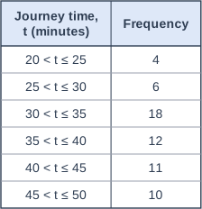
The table shows the journey times, t minutes, of 61 people who travel to work in a city.

Lucas merges the classes into just two classes, \(20 < t \le 35\) and \(35 < t \le 50\).

Work out the frequency of each of Lucas's classes.
Explain why Lucas's table gives a misleading impression of where the most common journey times are.

Table with columns "Journey time, t (minutes)", "Frequency". Journey time, t (minutes): 20 < t ≤ 25; Frequency: 4 | Journey time, t (minutes): 25 < t ≤ 30; Frequency: 6 | Journey time, t (minutes): 30 < t ≤ 35; Frequency: 18 | Journey time, t (minutes): 35 < t ≤ 40; Frequency: 12 | Journey time, t (minutes): 40 < t ≤ 45; Frequency: 11 | Journey time, t (minutes): 45 < t ≤ 50; Frequency: 10.

Model answer

\(20 < t \le 35\): 4 + 6 + 18 = 28
\(35 < t \le 50\): 12 + 11 + 10 = 33
In the original table the modal class is \(30 < t \le 35\), with 18 people. In Lucas's table the modal class is \(35 < t \le 50\), which suggests that most journeys take more than 35 minutes.
Merging into two wide classes has hidden the peak at 30 to 35 minutes inside a class that also contains the few short journeys of 20 to 30 minutes, so the table no longer shows where the journey times are most concentrated.

Explanation

Merging classes makes a table simpler but loses information about the shape of the distribution. Here the original classes show a clear peak just below 35 minutes, but the two wide classes make the longer times look more common. Choose class widths that keep the main features of the data visible.

Mark scheme
  1. 1 mark

    B1 for 28 (for \(20 < t \le 35\)) and 33 (for \(35 < t \le 50\))

    Both needed. 28 = 4 + 6 + 18 and 33 = 12 + 11 + 10. The three marks are independent.

  2. 1 mark

    B1 for comparing the modal classes: in the original table the modal class is \(30 < t \le 35\) (frequency 18), but in Lucas's table the modal class is \(35 < t \le 50\), which does not contain it

    oe. ft their two frequencies for Lucas's modal class. Accept 'the original table shows the most common times are 30 to 35 minutes, but Lucas's table suggests they are over 35 minutes'.

  3. 1 mark

    B1 for explaining that merging into wide classes loses detail: the peak at 30 to 35 minutes is hidden inside the class \(20 < t \le 35\), which also contains the uncommon short times of 20 to 30 minutes (only 10 people)

    oe. Must refer to the detail (the peak, or the shape of the distribution) being lost by using wide classes, in context. Do not accept 'merging loses detail' with no reference to these journey times. Ignore any non-contradictory or irrelevant statements.

Question 4

4 marks

Ella's hypothesis is

'Students who eat breakfast score higher marks in a morning test than students who do not eat breakfast.'

Write down the explanatory variable and the response variable, and state the type of data each one gives.
Ella plans to show her data on a scatter diagram. Explain why a scatter diagram is not suitable, and suggest a better way of comparing the data.

Model answer

Explanatory variable: whether the student eats breakfast (yes or no) - this is qualitative (categorical) data.
Response variable: the student's test mark - this is quantitative (discrete) data.
A scatter diagram needs two numerical variables. Whether a student eats breakfast is a category, not a number, so it cannot be plotted against the marks to show a correlation.
Ella should split the marks into the two groups, work out the median and the interquartile range of the marks for each group, and draw box plots of the two groups on the same scale. If the median mark of the breakfast group is higher, the data support her hypothesis.

Explanation

The type of data decides the analysis. When the explanatory variable is categorical, the data form groups to compare (with averages, spreads and comparative diagrams such as box plots); scatter diagrams and correlation are only for two numerical variables. Hypotheses that compare groups are very common, so check the type of each variable before choosing a diagram.

Mark scheme
  1. 1 mark

    B1 for explanatory variable: whether the student eats breakfast, and response variable: the test mark

    Both needed, the right way round. Accept 'independent variable' and 'dependent variable'. The four marks are independent.

  2. 1 mark

    B1 for whether the student eats breakfast is qualitative (categorical) data, and the test mark is quantitative (discrete) data

    Both needed. Accept 'categorical' or 'qualitative' for breakfast (yes / no) and 'quantitative', 'numerical' or 'discrete' for the mark. Condone 'continuous' for the mark only if 'quantitative' or 'numerical' is also given. ft if the variables are the wrong way round in the first mark point.

  3. 1 mark

    B1 for explaining that a scatter diagram needs two numerical variables, but whether a student eats breakfast is a category (yes or no), so it cannot show a correlation

    oe. Accept 'the breakfast data are not numbers, so they cannot be plotted against the marks on a scatter diagram'. Do not accept 'there is no correlation' or 'the data are not bivariate' with no reason.

  4. 1 mark

    B1 for a suitable way of comparing the two groups, eg work out the median (or mean) and the interquartile range (or range) of the marks for the students who eat breakfast and for those who do not, and compare them / draw box plots (or back-to-back stem-and-leaf diagrams) of the two groups' marks on the same scale

    oe. Must compare the marks of the two groups using an average or a suitable comparative diagram. Do not accept a pie chart, a bar chart of the number of students in each group, or 'compare the data' with no method.

Ready to try the rest? Every answer you write is marked against the mark scheme, so you can see exactly where the marks are.

Study Helper Hints first, answers after you try

Stuck on this one? Ask for a hint and I’ll point you in the right direction, without giving the answer away. Once you’ve checked your answer, I’ll show you how the marks are awarded.