
Level:
Correct: 0
Incorrect: 0
Marks: 0/0
Exam Practice
Course:
Topics:
AQA GCSE Statistics (Higher Paper 2) Smart practice A mixed round aimed at your weak spots
Unit 1
Planning and collecting data
Unit 2
Representing data
Section C: C1a (tabulation, tally, pictogram); Section E: E3d
Tabulation, tallies, pictograms and tables of data
Section C: C1a (pie chart), C1b (comparative pie chart)
Pie charts and comparative pie charts
Section C: C1a (stem and leaf diagram)
Stem and leaf diagrams
Section C: C2 (bar charts, bar line charts, line charts, frequency polygons)
Bar charts, line charts and frequency polygons
Section C: C2 (cumulative frequency charts)
Cumulative frequency diagrams
Section C: C2 (histograms), C3b
Histograms and frequency density
Section C: C2 (box plots); Section D: D3b; Section E: E5b
Box plots and outliers
Unit 3
Summarising data
Section D: D1a (mode, median, arithmetic mean)
Mode, median and mean
Section D: D1a (weighted mean, geometric mean), D1b
Weighted mean, geometric mean and choosing an average
Section D: D2; Section E: E5a
Skewness
Section D: D3a (range, quartiles, IQR, percentiles, interpercentile and interdecile range)
Range, quartiles, percentiles and interdecile range
Section D: D3a (standard deviation)
Standard deviation
Section C: C2 (time series); Section D: D1a (mean seasonal variation), D4; Section E: E6
Time series, moving averages and seasonal variation
Section C: C2 (scatter charts); Section D: D5
Scatter diagrams, lines of best fit and regression lines
Section D: D6; Section E: E9a, E9b, E9c
Spearman's rank correlation coefficient
Unit 4
Probability
Unit 5
Interpreting and evaluating results
Unit 6
Statistical enquiry cycle
3.6 Statistical enquiry cycle: 3.6.1 Initial planning, 3.6.2 Data collection
Statistical enquiry cycle: planning and data collection
3.6 Statistical enquiry cycle: 3.6.3 Processing and presentation, 3.6.4 Interpretation, 3.6.5 Evaluation
Statistical enquiry cycle: analysis and evaluation
Avg
score:
–
Topics
done:
0/39

Choosing representations and misleading diagrams

Practise 15 exam-style questions on Choosing representations and misleading diagrams for AQA GCSE Statistics (Higher Paper 2). Write your answer as you would in the exam and get it marked in seconds against the mark scheme, point by point, with the Study Helper on hand if you get stuck.

  • 15 questions
  • 1–5 marks each
  • Instant marking
  • No sign-up needed
15 questions, marked as you go

Sample questions with model answers

Here are 4 of the questions in this topic, each with a model answer, an explanation of why it earns the marks and the mark scheme an examiner would use.

Question 1

1 mark

Which of these can be found from a box plot and also from a cumulative frequency graph?

Choose your answer.

  • the mean
  • the interquartile range
  • the mode
  • the standard deviation

Model answer

The interquartile range
A box plot shows the lower and upper quartiles as the ends of the box, and both quartiles can be read from a cumulative frequency graph, so the interquartile range can be found from either diagram.

Explanation

Different diagrams show different summary values. A box plot shows only the lowest value, the quartiles, the median and the highest value, so any measure that needs all the values, such as the mean or standard deviation, cannot be found from it. Being able to extract the same measure from two formats is what allows data sets shown in different ways to be compared.

Mark scheme
  1. 1 mark

    B1 for the interquartile range

    Accept IQR. Any other answer, or more than one answer, scores B0. On a box plot the IQR is the length of the box; on a cumulative frequency graph it is the upper quartile minus the lower quartile, read at 3n/4 and n/4. The mean, the mode and the standard deviation cannot be found from a box plot.
Question 2

2 marks

A road safety group published a line graph showing the number of road accidents in a town each year from 2016 to 2025.
On the vertical axis of the graph, 0 is at the top and the numbers get larger going down the axis.
On the graph, the line goes down from 2016 to 2020 and then goes up from 2020 to 2025.

A reader says,
"The number of accidents has been increasing since 2020, because the line goes up after 2020."

Explain why the reader is wrong.
Describe how the number of accidents changed from 2016 to 2025.

Model answer

The vertical axis is upside down: 0 is at the top and larger numbers are lower down the page. So when the line goes up the page, the number of accidents is getting smaller. The rise in the line after 2020 shows that the number of accidents has been falling since 2020, not increasing.

The number of accidents increased from 2016 to 2020, when it was at its highest, and then decreased from 2020 to 2025.

Explanation

Readers expect larger values to be higher up a graph, so reversing a scale makes every rise look like a fall and every fall look like a rise. Always read the numbers on the axes before describing a trend. This is an example of an incorrect scale causing a graphical misrepresentation.

Mark scheme
  1. 1 mark

    B1 for the vertical axis is upside down (the numbers get larger going down), so a line going up the graph shows the number of accidents decreasing: accidents have fallen since 2020

    oe, eg 'higher up the graph means fewer accidents'; 'the scale is reversed, so the rise in the line is really a fall'. The answer must refer to the reversed (upside-down) vertical scale and what it does to the direction of the line. 'The axis does not start at 0', 'the scale is wrong' or 'the graph is misleading' with no explanation scores B0.

  2. 1 mark

    B1 for the number of accidents increased from 2016 to 2020 (it was highest in 2020) and then decreased from 2020 to 2025

    oe. Both parts of the change are needed (up to 2020, then down after 2020). 'The number of accidents went down from 2016 to 2020 and then up' (reading the graph the normal way) scores B0. Ignore any non-contradictory or irrelevant statements.

Question 3

3 marks

A supermarket's leaflet shows the number of single-use plastic bags it gave out in 2015 and in 2025 as two bars.
In 2015 it gave out 1.2 million bags. In 2025 it gave out 0.3 million bags.
The bar for 2025 is drawn a quarter of the height of the bar for 2015, and it is also half as wide.

Explain why the leaflet is misleading.
The bar for 2015 represents 1.2 million bags. Work out the number of bags that the area of the bar for 2025 suggests.

Model answer

The heights are correct: 0.3 million is a quarter of 1.2 million, and the 2025 bar is a quarter as tall. But the 2025 bar is also half as wide, so its area is \(\dfrac{1}{4} \times \dfrac{1}{2} = \dfrac{1}{8}\) of the area of the 2015 bar. Readers see the size of the bars, so the fall looks much bigger than it was.
Number suggested by the area of the 2025 bar \(= 1.2 \times \dfrac{1}{8} = 0.15\) million = 150 000 bags (the true number is 300 000).

Explanation

In a bar chart every bar should be the same width, so that only the heights change and the areas are in the same ratio as the values. Changing the width as well multiplies the visual effect: here a fall to a quarter looks like a fall to an eighth. Pictures that are scaled in two directions exaggerate changes in the same way.

Mark scheme
  1. 1 mark

    B1 for the 2025 bar has also been made narrower, so its area is much less than a quarter of the area of the 2015 bar, which makes the fall in the number of bags look bigger than it really was

    oe, eg 'the bars should be the same width: only the heights should change'; 'the 2025 bar looks like an eighth of the 2015 bar, but the number of bags fell to a quarter'. The answer must refer to the width (or the area) of the 2025 bar and its effect on the impression given. 'The bars are different widths' with no effect, or 'the heights are wrong', scores B0. The heights are in the correct proportion (\(\dfrac{0.3}{1.2} = \dfrac{1}{4}\)).

  2. 1 mark

    M1 for \(\dfrac{1}{4} \times \dfrac{1}{2}\) or \(\dfrac{1}{8}\) or 0.125 as the ratio of the areas of the bars

    oe, eg \(1.2 \times \dfrac{1}{4} \times \dfrac{1}{2}\). Using only the height (\(\dfrac{1}{4}\), giving 0.3 million) or only the width (\(\dfrac{1}{2}\), giving 0.6 million) is not a correct method: M0.

  3. 1 mark

    A1 for 150 000 (bags) or 0.15 million

    Correct answer with no working scores M1A1. 0.3 million (the true number) scores M0A0.

Question 4

4 marks

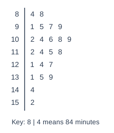
A film festival showed 23 films. The stem-and-leaf diagram shows the lengths, in minutes, of these films.

A streaming service has 60 films in its 'New releases' section. Their lengths, \(t\) minutes, are summarised here.

\(80 < t \le 90\): 6 films   \(90 < t \le 100\): 14 films   \(100 < t \le 110\): 18 films
\(110 < t \le 120\): 12 films   \(120 < t \le 140\): 8 films   \(140 < t \le 160\): 2 films

Compare the median lengths of the films at the festival and the films in the 'New releases' section.

Stem and leaf diagram. Key: 8 | 4 means 84 minutes. Rows (stem | leaves): 8 | 4 8; 9 | 1 5 7 9; 10 | 2 4 6 8 9; 11 | 2 4 5 8; 12 | 1 4 7; 13 | 1 5 9; 14 | 4; 15 | 2.

Model answer

Festival: n = 23, so the median is the 12th value = 112 minutes.
Streaming service: n = 60, so the median is the 30th value.
Cumulative frequencies: 6, 20, 38, ... so the median is in the class \(100 < t \le 110\).
Median ≈ \(100 + \dfrac{30 - 20}{18} \times 10 = 105.6\) minutes
On average, the films at the festival were longer than the 'New releases' films (median 112 minutes compared with about 105.6 minutes).

Explanation

To compare data in two formats, find the same measure from each: the exact median from the ordered stem-and-leaf diagram, and an estimate of the median by interpolation from the grouped data. Then compare in context. The grouped median is only an estimate, because the exact lengths in each class are not known.

Mark scheme
  1. 1 mark

    B1 for festival median 112 (minutes)

    The 12th value of the ordered data.

  2. 1 mark

    M1 for \(100 + \dfrac{30 - 20}{18} \times 10\) or \(100 + \dfrac{30.5 - 20}{18} \times 10\)

    oe. The median is the 30th (or 30.5th) value, in the class \(100 < t \le 110\) (cumulative frequencies 6, 20, 38, ...).

  3. 1 mark

    A1 for streaming median 105.6 [105.5, 105.9]

    105.55... from the 30th value; 105.83... from the 30.5th value. The midpoint of the median class (105) A0.

  4. 1 mark

    B1ft for a correct comparison in context, eg on average the festival films were longer than the 'New releases' films

    ft their medians, but comparison marks cannot be awarded unless both medians have been worked out. Must include 'on average' / 'generally' / 'typically' or an interpretation of the median, and context (length / films). 'The festival median is higher' with no interpretation B0. Comparing means B0. Any values stated must be correct. Ignore any non-contradictory or irrelevant statements.

Ready to try the rest? Every answer you write is marked against the mark scheme, so you can see exactly where the marks are.

Study Helper Hints first, answers after you try

Stuck on this one? Ask for a hint and I’ll point you in the right direction, without giving the answer away. Once you’ve checked your answer, I’ll show you how the marks are awarded.