
Level:
Correct: 0
Incorrect: 0
Marks: 0/0
Exam Practice
Course:
Topics:
AQA GCSE Statistics (Higher Paper 2) Smart practice A mixed round aimed at your weak spots
Unit 1
Planning and collecting data
Unit 2
Representing data
Section C: C1a (tabulation, tally, pictogram); Section E: E3d
Tabulation, tallies, pictograms and tables of data
Section C: C1a (pie chart), C1b (comparative pie chart)
Pie charts and comparative pie charts
Section C: C1a (stem and leaf diagram)
Stem and leaf diagrams
Section C: C2 (bar charts, bar line charts, line charts, frequency polygons)
Bar charts, line charts and frequency polygons
Section C: C2 (cumulative frequency charts)
Cumulative frequency diagrams
Section C: C2 (histograms), C3b
Histograms and frequency density
Section C: C2 (box plots); Section D: D3b; Section E: E5b
Box plots and outliers
Unit 3
Summarising data
Section D: D1a (mode, median, arithmetic mean)
Mode, median and mean
Section D: D1a (weighted mean, geometric mean), D1b
Weighted mean, geometric mean and choosing an average
Section D: D2; Section E: E5a
Skewness
Section D: D3a (range, quartiles, IQR, percentiles, interpercentile and interdecile range)
Range, quartiles, percentiles and interdecile range
Section D: D3a (standard deviation)
Standard deviation
Section C: C2 (time series); Section D: D1a (mean seasonal variation), D4; Section E: E6
Time series, moving averages and seasonal variation
Section C: C2 (scatter charts); Section D: D5
Scatter diagrams, lines of best fit and regression lines
Section D: D6; Section E: E9a, E9b, E9c
Spearman's rank correlation coefficient
Unit 4
Probability
Unit 5
Interpreting and evaluating results
Unit 6
Statistical enquiry cycle
3.6 Statistical enquiry cycle: 3.6.1 Initial planning, 3.6.2 Data collection
Statistical enquiry cycle: planning and data collection
3.6 Statistical enquiry cycle: 3.6.3 Processing and presentation, 3.6.4 Interpretation, 3.6.5 Evaluation
Statistical enquiry cycle: analysis and evaluation
Avg
score:
–
Topics
done:
0/39

Statistical enquiry cycle: analysis and evaluation

Practise 18 exam-style questions on Statistical enquiry cycle: analysis and evaluation for AQA GCSE Statistics (Higher Paper 2). Write your answer as you would in the exam and get it marked in seconds against the mark scheme, point by point, with the Study Helper on hand if you get stuck.

  • 18 questions
  • 1–6 marks each
  • Instant marking
  • No sign-up needed
18 questions, marked as you go

Sample questions with model answers

Here are 4 of the questions in this topic, each with a model answer, an explanation of why it earns the marks and the mark scheme an examiner would use.

Question 1

1 mark

Zara is testing the hypothesis 'Commuters who listen to music on the train feel less stressed than commuters who do not.'
One morning, she asked 12 commuters on one train to rate their stress from 1 to 10.

Which change would most improve the reliability of her conclusion?

Choose your answer.

  • Ask a larger random sample of commuters, on different trains and days
  • Give each group's mean stress rating to a greater degree of accuracy
  • Leave out any stress ratings that do not fit in with her hypothesis
  • Present her results in a 3D bar chart with a colour for each group

Model answer

Ask a larger random sample of commuters, on different trains and days

Explanation

Reliability improves with more data, collected so that it represents the population: a larger random sample, taken on different trains and days, reduces the effect of chance and of one unusual morning. Giving the means more accurately does not make the data more reliable, leaving out values that do not fit biases the results, and a 3D chart only changes the presentation (and can mislead).

Mark scheme
  1. 1 mark

    B1 for Ask a larger random sample of commuters, on different trains and days

    Accept any clear indication of this option. Any other answer, or more than one answer, scores B0.
Question 2

2 marks

A town council is testing the hypothesis 'Social media is the most common way that residents of the town get local news.'
It asked 200 residents how they mainly get local news, and typed each answer into a spreadsheet as a code:

1 = social media   2 = local newspaper   3 = local radio   4 = council website   5 = word of mouth

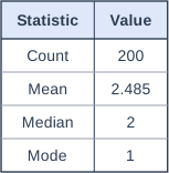
The table shows the spreadsheet's summary of the codes.

A council officer says,
'The mean code is 2.485, which rounds to 2, so a typical resident gets local news from the local newspaper. The hypothesis is not supported.'

Explain why the officer's method is not valid.
Use the table to decide whether the results support the hypothesis.

Table with columns "Statistic", "Value". Statistic: Count; Value: 200 | Statistic: Mean; Value: 2.485 | Statistic: Median; Value: 2 | Statistic: Mode; Value: 1.

Model answer

The numbers 1 to 5 are only labels for the ways of getting local news (categorical data), not amounts. A mean code of 2.485 has no meaning: numbering the categories in a different order would give a different mean, so it cannot show how a typical resident gets local news.

For categorical data the suitable average is the mode. The mode is 1, which is social media, so social media is the most common way that the residents asked get local news. The results support the hypothesis.

Explanation

Coding answers as numbers makes them quick to type and count, but a spreadsheet will work out a mean, a median or a standard deviation of any numbers, even when they are only labels. For categorical data only the mode, or the number or percentage in each category, has a meaning, and the mode is exactly what a 'most common' hypothesis needs.

Mark scheme
  1. 1 mark

    B1 for the codes are only labels for categories (qualitative data), not amounts, so the mean of the codes has no meaning / numbering the ways of getting news in a different order would give a different mean

    oe. Accept 'you cannot find the mean of categorical data'. 'The mean is wrong' B0 (2.485 is the correct mean of the codes). 'The officer should use the median' B0 (the median of the codes has no meaning either). 'The mean is affected by extreme values' B0. 'The officer should not round 2.485' B0.

  2. 1 mark

    B1 for the mode is 1 (social media), so social media is the most common way that residents get local news and the results support the hypothesis

    Must use the mode (or say that code 1 is the most common answer) and give a decision. 'Yes' alone B0. A decision based on the mean or the median B0. Ignore a correct comment that the mode does not show whether more than half of the residents use social media.

Question 3

3 marks

A shop owner is testing the hypothesis 'Customers spend more time in the shop on days when music is played.'
One Monday, with music playing, she timed 9 customers. The next day, with no music, she timed another 9 customers.

With music: median 14 minutes, interquartile range 11 minutes
No music: median 13 minutes, interquartile range 12 minutes

She concludes that her hypothesis is correct.
Use the medians and interquartile ranges to explain why these results give very little evidence for her hypothesis.
Give one other weakness of her method, and describe how she should change her method to deal with it.

Model answer

The median time with music is only 1 minute longer, but the interquartile ranges are 11 and 12 minutes, so the times in the two groups overlap a lot. A difference of 1 minute could easily happen by chance with a different 9 customers, so it is very little evidence that music makes customers stay longer.

Other weakness: she timed customers on only one day with music and one day without, and a Monday and a Tuesday may differ in other ways, such as how busy the shop was.

Change: collect data over several weeks, playing music on randomly chosen days and not on others, time many more customers, and compare the times for the same days of the week.

Explanation

A difference between two averages is only convincing when it is large compared with the spread of the data and the samples are large. With small samples, the medians would change from one sample to the next, so a 1-minute difference shows very little. Collecting data over many days, with the music days chosen at random, also stops other differences between days affecting the result.

Mark scheme
  1. 1 mark

    B1 for the difference between the medians (1 minute) is very small compared with the spread of the times (interquartile ranges of 11 and 12 minutes), so the two sets of times overlap a lot and the difference could easily be due to chance (sampling variation)

    oe. Must use both the size of the difference in medians and the spread. Accept 'the medians differ by only 1 minute, but the middle half of the times spreads over 11 or 12 minutes, so another 9 customers could easily give the opposite result'. 'The medians are close' with no reference to the spread B0. 'The music median is higher' B0.

  2. 1 mark

    B1 for another weakness, eg only 9 customers each day is a small sample / she collected data on only one day for each, and the two days may differ in other ways (eg how busy the shop was, the weather, or the type of shoppers on a Monday and on a Tuesday)

    oe. Must be different from the first point (not just the size of the difference). 'It is biased' with no reason B0.

  3. 1 mark

    B1dep for a change that deals with their weakness, eg time many more customers (small sample) / collect data over several weeks, playing music on randomly chosen days, and compare the same days of the week (one day each)

    Dependent on the previous mark: the change must deal with the weakness given. Must be specific, eg more customers or more days, or choosing the music days at random. 'Ask more people' B0 unless it says time more customers. 'Do it again' alone B0.

Question 4

4 marks

Jack is testing the hypothesis 'Cars that are more than 10 years old are more likely to break down than newer cars.'
A breakdown company covers 40 000 cars. 10 000 of these cars are more than 10 years old.
Last year, the company was called out to 6000 breakdowns of these cars. 2100 of the breakdowns were of cars more than 10 years old.

Jack says,
'Only 35% of the breakdowns were of cars more than 10 years old, so newer cars break down more often. My hypothesis is not supported.'

Explain why Jack's reasoning is wrong.
Use the figures to decide whether the data support his hypothesis.
You must show your working.

Model answer

35% is the share of all the breakdowns that were of older cars. It is not the chance that an older car breaks down. Three-quarters of the cars (30 000 of the 40 000) are newer, so newer cars would have more breakdowns in total even if each newer car were less likely to break down. Jack needs to compare the breakdowns with the number of cars of each age.

Older cars: \(\dfrac{2100}{10000} = 0.21\) breakdowns per car
Newer cars: \(\dfrac{6000 - 2100}{40000 - 10000} = \dfrac{3900}{30000} = 0.13\) breakdowns per car

Older cars had 0.21 breakdowns per car, compared with 0.13 for newer cars, so cars more than 10 years old are more likely to break down. The data support Jack's hypothesis.

Explanation

To decide which group is more likely to have something happen, compare rates within each group (the number of breakdowns divided by the number of cars in that group), not each group's share of all the cases. A group that makes up most of the population can have most of the cases even when its rate is lower. A quick check is to compare each group's share of the cases with its share of the population: older cars are 25% of the cars but had 35% of the breakdowns.

Mark scheme
  1. 1 mark

    B1 for an explanation, eg 35% is the share of the breakdowns, not the chance that an older car breaks down: three-quarters of the cars (30 000) are newer, so newer cars could have more breakdowns in total even if each newer car is less likely to break down; the breakdowns must be compared with the number of cars of each age

    oe. Must refer to the different numbers of older and newer cars, or to comparing the breakdowns relative to the number of cars in each group. 'He has worked out the percentage wrongly' B0 (35% is correct). 'The sample is too small' B0.

  2. 1 mark

    M1 for a correct method for the breakdowns per car for one age group, eg \(\dfrac{2100}{10000}\) or \(\dfrac{6000 - 2100}{40000 - 10000}\)

    oe. Alternative method: the percentage of the cars that are more than 10 years old, \(\dfrac{10000}{40000}\) (= 25%), to compare with the 35% of the breakdowns.

  3. 1 mark

    A1 for 0.21 (21%) and 0.13 (13%) breakdowns per car, for older and newer cars

    oe, eg 21 and 13 breakdowns per 100 cars, or 2100 out of 10 000 and 3900 out of 30 000 written in a comparable form. Alternative method: 25% of the cars and 35% of the breakdowns are older cars, both seen.

  4. 1 mark

    B1ft for Yes, the data support the hypothesis, because older cars had more breakdowns per car than newer cars (0.21 compared with 0.13), or because older cars are 25% of the cars but had 35% of the breakdowns

    ft their values, provided they are rates (or shares) in a comparable form. Must give a decision. Comparing numbers of breakdowns (2100 and 3900) B0. The question says 'You must show your working': a decision with no working scores B0.

Ready to try the rest? Every answer you write is marked against the mark scheme, so you can see exactly where the marks are.

Study Helper Hints first, answers after you try

Stuck on this one? Ask for a hint and I’ll point you in the right direction, without giving the answer away. Once you’ve checked your answer, I’ll show you how the marks are awarded.