
Level:
Correct: 0
Incorrect: 0
Marks: 0/0
Exam Practice
Course:
Topics:
AQA GCSE Statistics (Higher Paper 2) Smart practice A mixed round aimed at your weak spots
Unit 1
Planning and collecting data
Unit 2
Representing data
Section C: C1a (tabulation, tally, pictogram); Section E: E3d
Tabulation, tallies, pictograms and tables of data
Section C: C1a (pie chart), C1b (comparative pie chart)
Pie charts and comparative pie charts
Section C: C1a (stem and leaf diagram)
Stem and leaf diagrams
Section C: C2 (bar charts, bar line charts, line charts, frequency polygons)
Bar charts, line charts and frequency polygons
Section C: C2 (cumulative frequency charts)
Cumulative frequency diagrams
Section C: C2 (histograms), C3b
Histograms and frequency density
Section C: C2 (box plots); Section D: D3b; Section E: E5b
Box plots and outliers
Unit 3
Summarising data
Section D: D1a (mode, median, arithmetic mean)
Mode, median and mean
Section D: D1a (weighted mean, geometric mean), D1b
Weighted mean, geometric mean and choosing an average
Section D: D2; Section E: E5a
Skewness
Section D: D3a (range, quartiles, IQR, percentiles, interpercentile and interdecile range)
Range, quartiles, percentiles and interdecile range
Section D: D3a (standard deviation)
Standard deviation
Section C: C2 (time series); Section D: D1a (mean seasonal variation), D4; Section E: E6
Time series, moving averages and seasonal variation
Section C: C2 (scatter charts); Section D: D5
Scatter diagrams, lines of best fit and regression lines
Section D: D6; Section E: E9a, E9b, E9c
Spearman's rank correlation coefficient
Unit 4
Probability
Unit 5
Interpreting and evaluating results
Unit 6
Statistical enquiry cycle
3.6 Statistical enquiry cycle: 3.6.1 Initial planning, 3.6.2 Data collection
Statistical enquiry cycle: planning and data collection
3.6 Statistical enquiry cycle: 3.6.3 Processing and presentation, 3.6.4 Interpretation, 3.6.5 Evaluation
Statistical enquiry cycle: analysis and evaluation
Avg
score:
–
Topics
done:
0/39

Experimental and theoretical probability and bias

Practise 13 exam-style questions on Experimental and theoretical probability and bias for AQA GCSE Statistics (Higher Paper 2). Write your answer as you would in the exam and get it marked in seconds against the mark scheme, point by point, with the Study Helper on hand if you get stuck.

  • 13 questions
  • 1–5 marks each
  • Instant marking
  • No sign-up needed
13 questions, marked as you go

Sample questions with model answers

Here are 4 of the questions in this topic, each with a model answer, an explanation of why it earns the marks and the mark scheme an examiner would use.

Question 1

1 mark

A fair six-sided dice is rolled many times. Here are four statements.

A   In 60 rolls, the dice will land on 6 exactly 10 times.
B   The relative frequency of 6 after 600 rolls is likely to be closer to \(\dfrac{1}{6}\) than the relative frequency after 60 rolls.
C   If the dice lands on 6 in 3 of its first 6 rolls, it must be biased.
D   Rolling the dice more times makes the probability of a 6 on each roll closer to \(\dfrac{1}{6}\).

Which statement is true?

Choose your answer.

  • A
  • B
  • C
  • D

Model answer

B
As the number of rolls increases, the relative frequency of 6 tends to get closer to the theoretical probability \(\dfrac{1}{6}\), so it is likely to be closer after 600 rolls than after 60 rolls.

Explanation

Experimental probability (relative frequency) tends towards the theoretical probability as the number of trials increases. The theoretical probability itself never changes, and an expected frequency such as 10 sixes in 60 rolls is an average, not a guaranteed result. A few rolls can easily give an unusual result, even with a fair dice.

Mark scheme
  1. 1 mark

    B1 for B

    Accept the statement written out instead of the letter. Relative frequency tends towards the theoretical probability as the number of trials increases. A is false: 10 is the expected number, but the actual number varies. C is false: 6 rolls are far too few to show bias. D is false: the probability of a 6 is \(\dfrac{1}{6}\) on every roll; it is the relative frequency that gets closer to \(\dfrac{1}{6}\). Any other answer, or more than one answer, scores B0.

Question 2

2 marks

A computer program simulates flipping a fair coin.
The table shows the number of heads after different numbers of flips.

Describe what happens to the relative frequency of heads as the number of flips increases.
Use values from the table in your answer.

Table with columns "Number of flips", "10", "100", "1000", "10 000". Number of flips: Number of heads; 10: 7; 100: 46; 1000: 512; 10 000: 4986.

Model answer

Relative frequencies: 10 flips \(\dfrac{7}{10} = 0.7\); 100 flips \(\dfrac{46}{100} = 0.46\); 1000 flips \(\dfrac{512}{1000} = 0.512\); 10 000 flips \(\dfrac{4986}{10\,000} = 0.4986\)
As the number of flips increases, the relative frequency gets closer to 0.5, the theoretical probability of heads for a fair coin: it is 0.7 after 10 flips but 0.4986 after 10 000 flips.

Explanation

When every trial is random and carried out in the same way, the relative frequency tends towards the theoretical probability as the number of trials increases. Notice that the number of heads does not get closer to the number of tails (the difference grows from 4 to 28): it is the proportion of heads that gets closer to 0.5.

Mark scheme
  1. 1 mark

    B1 for at least three correct relative frequencies from 0.7, 0.46, 0.512 and 0.4986

    oe, eg 70%, 46%, 51.2%, 49.86%. Accept 0.499 or 0.5 for 0.4986.

  2. 1 mark

    B1 for the relative frequency gets closer to 0.5 (the theoretical probability of heads) as the number of flips increases

    oe, eg 'it settles down at about 0.5', 'it varies a lot at first but tends towards 0.5'. Must mention 0.5 (or \(\dfrac{1}{2}\), or the theoretical probability). Do not accept 'the number of heads gets closer to the number of tails' (the difference between them actually grows, from 4 to 28) or 'it goes up and down' on its own. Ignore any non-contradictory or irrelevant statements.

Question 3

3 marks

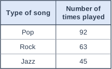
Lily's music app has a playlist of 40 songs. Each song is pop, rock or jazz.
In random play, each time a song ends the app chooses one of the 40 songs at random to play next, so a song can be played more than once.
Lily records the type of each of the next 200 songs that are played. The table shows her results.

Estimate the number of songs of each type in the playlist.

Lily says,

"There must be exactly 9 jazz songs in the playlist."

Comment on Lily's statement.

Table with columns "Type of song", "Number of times played". Type of song: Pop; Number of times played: 92 | Type of song: Rock; Number of times played: 63 | Type of song: Jazz; Number of times played: 45.

Model answer

Each play is a random choice from the 40 songs, so the relative frequency of each type estimates the fraction of the playlist of that type.
Pop: \(\dfrac{92}{200} \times 40 = 18.4\), so about 18 songs
Rock: \(\dfrac{63}{200} \times 40 = 12.6\), so about 13 songs
Jazz: \(\dfrac{45}{200} \times 40 = 9\) songs
(Check: 18 + 13 + 9 = 40)
Lily cannot be sure. 9 is the best estimate, but the plays are random, so the numbers vary by chance: with 8 or 10 jazz songs she would expect 40 or 50 jazz plays, and getting 45 would not be surprising. She would need to look at the playlist to know.

Explanation

The relative frequency from many random plays estimates the theoretical probability of a jazz song, which is the number of jazz songs divided by 40, so multiply each relative frequency by 40 and round to whole numbers that add up to 40. A relative frequency is only an estimate: even from 200 plays, results vary by chance, so the true number of jazz songs could be a little different from 9.

Mark scheme
  1. 1 mark

    M1 for a relative frequency \(\times\) 40 for one type, eg \(\dfrac{92}{200} \times 40\) (= 18.4), \(\dfrac{63}{200} \times 40\) (= 12.6) or \(\dfrac{45}{200} \times 40\) (= 9)

    oe, eg \(0.46 \times 40\), \(92 \div 5\), \(\dfrac{92}{200} = \dfrac{n}{40}\).

  2. 1 mark

    A1 for pop 18, rock 13 and jazz 9

    All three needed, as whole numbers of songs (they add up to 40). 18.4, 12.6 and 9 left as decimals scores M1A0. The numbers of plays (92, 63 and 45) or the percentages (46%, 31.5% and 22.5%) with no conversion to numbers of songs score M0A0. Correct answers with no working score M1A1.

  3. 1 mark

    B1 for Lily cannot be sure: 9 is only an estimate, because the numbers of plays vary by chance, so the playlist could have a different number of jazz songs (eg 8 or 10)

    oe, eg 'not necessarily - with 10 jazz songs she would expect 50 jazz plays, and 45 could easily happen', 'she would need to look at the playlist, or record many more plays, to be more certain'. Must say that the result is an estimate or that she cannot be certain, with a reason about chance (natural variation) or the number of plays. 'Yes, because \(\dfrac{45}{200} \times 40 = 9\)' scores B0. Ignore any non-contradictory or irrelevant statements.

Question 4

4 marks

Zoe wants to estimate the probability that a plastic bottle top lands with its open side facing up when it is dropped.

Describe how Zoe could carry out an experiment to estimate this probability.
In your answer, explain how she should make sure her results are not biased, and how she should use her results.

Model answer

Zoe should drop the same bottle top a large number of times, for example 200 times.
She should drop it from the same height (say 1 metre) onto the same surface each time, so the conditions do not change.
Before each drop she should shake it in a cupped hand, so that it does not always start the same way up and the result of each drop is random.
She should record whether it lands open side up each time, then estimate the probability as
number of times open side up \(\div\) 200 (the relative frequency).

Explanation

An experimental probability is only a good estimate of the theoretical probability when there are many trials, all carried out in the same way, and each trial is random. Changing the height or surface, or always dropping the top from the same starting position, could bias the results. The estimate is the relative frequency: the number of successes divided by the number of trials.

Mark scheme
  1. 1 mark

    B1 for dropping the bottle top a large number of times, eg at least 100 times

    oe, eg 'repeat it many times, because more trials give a more reliable estimate'. A number of trials, if given, must be at least 50. 'Drop it a few times' scores B0.

  2. 1 mark

    B1 for keeping the conditions the same for every drop, eg the same height and the same surface

    oe. At least one named condition (height, surface, the same bottle top) is needed. 'Make it a fair test' on its own scores B0.

  3. 1 mark

    B1 for making each drop random, eg shaking the bottle top in a cupped hand before each drop / not always starting with it the same way up

    oe. Must describe how the release is made random, so that the starting position does not affect the result. 'Make sure it is random' with no detail scores B0.

  4. 1 mark

    B1 for the estimate = number of times it lands open side up \(\div\) total number of drops (the relative frequency)

    oe, eg 'record the results in a tally chart and work out the relative frequency'. Must say how the estimate is calculated. 'Record the results' on its own scores B0. 1 mark for each different feature, max 4. The same feature given twice scores only once. Ignore any non-contradictory or irrelevant statements.

Ready to try the rest? Every answer you write is marked against the mark scheme, so you can see exactly where the marks are.

Study Helper Hints first, answers after you try

Stuck on this one? Ask for a hint and I’ll point you in the right direction, without giving the answer away. Once you’ve checked your answer, I’ll show you how the marks are awarded.