Level:
Correct: 0
Incorrect: 0
Marks: 0/0
Exam Practice
Course:
Topics:
AQA GCSE Statistics (Higher Paper 2) Smart practice A mixed round aimed at your weak spots
Unit 1
Planning and collecting data
Unit 2
Representing data
Section C: C1a (tabulation, tally, pictogram); Section E: E3d
Tabulation, tallies, pictograms and tables of data
Section C: C1a (pie chart), C1b (comparative pie chart)
Pie charts and comparative pie charts
Section C: C1a (stem and leaf diagram)
Stem and leaf diagrams
Section C: C2 (bar charts, bar line charts, line charts, frequency polygons)
Bar charts, line charts and frequency polygons
Section C: C2 (cumulative frequency charts)
Cumulative frequency diagrams
Section C: C2 (histograms), C3b
Histograms and frequency density
Section C: C2 (box plots); Section D: D3b; Section E: E5b
Box plots and outliers
Unit 3
Summarising data
Section D: D1a (mode, median, arithmetic mean)
Mode, median and mean
Section D: D1a (weighted mean, geometric mean), D1b
Weighted mean, geometric mean and choosing an average
Section D: D2; Section E: E5a
Skewness
Section D: D3a (range, quartiles, IQR, percentiles, interpercentile and interdecile range)
Range, quartiles, percentiles and interdecile range
Section D: D3a (standard deviation)
Standard deviation
Section C: C2 (time series); Section D: D1a (mean seasonal variation), D4; Section E: E6
Time series, moving averages and seasonal variation
Section C: C2 (scatter charts); Section D: D5
Scatter diagrams, lines of best fit and regression lines
Section D: D6; Section E: E9a, E9b, E9c
Spearman's rank correlation coefficient
Unit 4
Probability
Unit 5
Interpreting and evaluating results
Unit 6
Statistical enquiry cycle
3.6 Statistical enquiry cycle: 3.6.1 Initial planning, 3.6.2 Data collection
Statistical enquiry cycle: planning and data collection
3.6 Statistical enquiry cycle: 3.6.3 Processing and presentation, 3.6.4 Interpretation, 3.6.5 Evaluation
Statistical enquiry cycle: analysis and evaluation
Avg
score:
–
Topics
done:
0/39

Skewness

Practise 14 exam-style questions on Skewness for AQA GCSE Statistics (Higher Paper 2). Write your answer as you would in the exam and get it marked in seconds against the mark scheme, point by point, with the Study Helper on hand if you get stuck.

  • 14 questions
  • 1–6 marks each
  • Instant marking
  • No sign-up needed
14 questions, marked as you go

Sample questions with model answers

Here are 4 of the questions in this topic, each with a model answer, an explanation of why it earns the marks and the mark scheme an examiner would use.

Question 1

1 mark

Which of these sets of data is most likely to have negative skew?

Choose your answer.

  • the marks in a test that most students found very easy
  • the prices of the houses in a town
  • the shoe sizes of adult men
  • the numbers of children in families

Model answer

The marks in a test that most students found very easy.
Most students score close to full marks and no one can score more, but a few students score much lower, giving a tail of low marks: negative skew.

Explanation

Negative skew happens when the values are bunched near an upper limit with a tail of a few much lower values, so the mean is below the median. Prices and counts such as numbers of children are bunched near the lower end with a few very large values, which is positive skew, while the shoe sizes of adult men are roughly symmetrical.

Mark scheme
  1. 1 mark

    B1 for the marks in a test that most students found very easy

    Accept any clear indication of this option. Most marks are high (they cannot go above full marks), with a tail of a few low marks. House prices and numbers of children usually have positive skew (a few very large values), and the shoe sizes of adult men are roughly symmetrical. Any other answer, or more than one answer, scores B0.
Question 2

2 marks

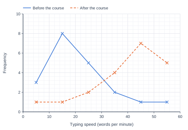
20 students took a typing test before and after a typing course.
The frequency polygons show their typing speeds, in words per minute.

Describe the skew of the typing speeds before the course and the skew of the typing speeds after the course.

Line graph of frequency (y-axis, 0 to 10) against typing speed (words per minute) (x-axis, 0 to 60). "Before the course" joins the points (5, 3), (15, 8), (25, 5), (35, 2), (45, 1), (55, 1). "After the course" (dashed) joins the points (5, 1), (15, 1), (25, 2), (35, 4), (45, 7), (55, 5).

Model answer

Before the course: positive skew. Most students typed between 10 and 30 words per minute, with a tail of a few faster typists.
After the course: negative skew. Most students typed between 40 and 60 words per minute, with a tail of a few slower typists.

Explanation

On a frequency polygon, look at where the peak is and which way the long tail stretches. A peak at the low values with a tail to the right is positive skew; a peak at the high values with a tail to the left is negative skew. Here the course has moved most students to the fast end.

Mark scheme
  1. 1 mark

    B1 for before the course: positive (skew)

    Accept 'skewed to the right' oe, or an interpretation, eg 'before the course most students typed slowly, with a few fast typists'. Ignore any reference to the degree of skewness.

  2. 1 mark

    B1 for after the course: negative (skew)

    Accept 'skewed to the left' oe, or 'after the course most students typed quickly, with a few slow typists'. Each skew must be clearly matched to before or after: 'one is positive and the other is negative' scores B0B0.

Question 3

3 marks

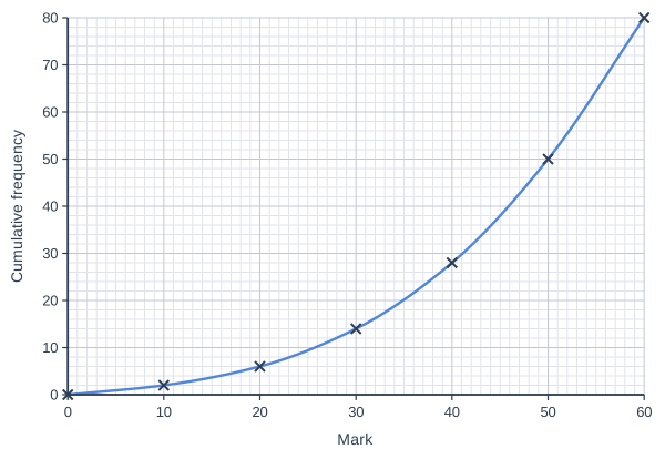
The cumulative frequency graph shows information about the marks scored by 80 students in a test.

Jess says,
"The graph is steepest at the right-hand end, so the marks have positive skew."

Use estimates of the median and the quartiles from the graph to decide whether Jess is correct.
Give a reason for your answer.

Cumulative frequency graph on a grid of small squares. The horizontal axis is "Mark", from 0 to 60, numbered every 10, with 10 small squares between numbered values (each small square is 1). The vertical axis is "Cumulative frequency", from 0 to 80, numbered every 10, with 5 small squares between numbered values (each small square is 2). A smooth curve starts at (0, 0) and passes through (10, 2), (20, 6), (30, 14), (40, 28), (50, 50) and (60, 80) (each point is marked with a cross).

Model answer

n = 80, so read across at 40 for the median, 20 for the lower quartile and 60 for the upper quartile.
Median ≈ 46, lower quartile ≈ 35, upper quartile ≈ 53.5
UQ - median ≈ 53.5 - 46 = 7.5 and median - LQ ≈ 46 - 35 = 11
The median is closer to the upper quartile, so the lower marks are more spread out: the marks have negative skew, and Jess is not correct.
The graph is steepest on the right because many students scored high marks; the long, shallow part on the left is a tail of low marks.

Explanation

The steepest part of a cumulative frequency graph shows where the data are most concentrated. A graph that is steepest at the right-hand end means most of the values are high, with a tail of lower values, which is negative skew. Comparing UQ - median with median - LQ confirms this: the lower half of the middle 50% of the marks is more spread out.

Mark scheme
  1. 1 mark

    B1 for median = 46 [45, 47]

    Read at a cumulative frequency of 40 (or 40.5). The drawn curve gives 45.9; joining the plotted points with straight lines gives 45.5. Both are in the range.

  2. 1 mark

    B1 for lower quartile = 35 [34, 36] and upper quartile = 53.5 [52.5, 54.5]

    Both needed. Read at cumulative frequencies of 20 and 60 (or 20.25 and 60.75). The drawn curve gives 34.9 and 53.6; straight lines between the plotted points give 34.3 and 53.3. All are in the ranges.

  3. 1 mark

    B1ft for Jess is not correct: the marks have negative skew, with a reason using the quartiles, eg the median is closer to the upper quartile than to the lower quartile / UQ - median is less than median - LQ

    ft their median and quartiles. Values in the ranges give negative skew unless the readings are at opposite ends of the ranges (eg LQ 36, median 45, UQ 54.5, where UQ - median is 9.5 and median - LQ is 9); a conclusion that follows correctly from their values scores B1ft. Accept values, eg 53.5 - 46 = 7.5 and 46 - 35 = 11. Accept 'the lower marks are more spread out than the higher marks' as the reason. 'Jess is wrong' or 'negative' with no reason from the quartiles scores B0. Ignore any reference to the degree of skewness.

Question 4

4 marks

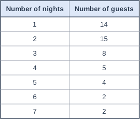
The table shows the numbers of nights that 50 guests stayed at a hotel.

The standard deviation of the numbers of nights is 1.65 (to 2 decimal places).

\(\text{skew} = \dfrac{3(\text{mean} - \text{median})}{\text{standard deviation}}\)

Work out the skew of the numbers of nights.
Give your answer to 2 decimal places.

Table with columns "Number of nights", "Number of guests". Number of nights: 1; Number of guests: 14 | Number of nights: 2; Number of guests: 15 | Number of nights: 3; Number of guests: 8 | Number of nights: 4; Number of guests: 5 | Number of nights: 5; Number of guests: 4 | Number of nights: 6; Number of guests: 2 | Number of nights: 7; Number of guests: 2.

Model answer

\(\sum fx = 1 \times 14 + 2 \times 15 + 3 \times 8 + 4 \times 5 + 5 \times 4 + 6 \times 2 + 7 \times 2 = 134\)
Mean \(= \dfrac{134}{50} = 2.68\) nights
Median: the 25th and 26th values. The cumulative frequencies are 14, 29, ... so both are 2. Median = 2 nights
\(\text{skew} = \dfrac{3(2.68 - 2)}{1.65} = \dfrac{2.04}{1.65} = 1.236...\)
Skew = 1.24 (to 2 decimal places)

Explanation

For a frequency table, the mean is the total number of nights divided by the number of guests, and the median is found by counting through the cumulative frequencies to the middle position. Common errors are finding the mean or the median of the frequencies instead of the numbers of nights. The positive skew fits the table: most guests stayed 1 or 2 nights, with a few staying much longer.

Mark scheme
  1. 1 mark

    B1 for (mean =) 2.68

    134 ÷ 50. Do not accept 4 (the mean of 1 to 7) or 7.14 (50 ÷ 7).

  2. 1 mark

    B1 for (median =) 2

    The 25th and 26th values are both 2 (cumulative frequencies 14, 29, ...). Do not accept 15 (a frequency) or 4.

  3. 1 mark

    M1 for \(\dfrac{3(2.68 - 2)}{1.65}\)

    ft their mean and median

  4. 1 mark

    A1 for 1.24 [1.23, 1.24]

    Accept more accurate values in the range, eg 1.236. 1.23 comes from using the unrounded standard deviation (1.6545...) worked out from the table, which is also accepted. Correct answer with no working scores full marks. Using the mean of the values 1 to 7 (4) gives 3.64: B0B1M1A0.

Ready to try the rest? Every answer you write is marked against the mark scheme, so you can see exactly where the marks are.

Study Helper Hints first, answers after you try

Stuck on this one? Ask for a hint and I’ll point you in the right direction, without giving the answer away. Once you’ve checked your answer, I’ll show you how the marks are awarded.