Graphs: choosing, plotting and reading them - AQA A-Level Biology (Paper 3) Exam Questions

Practise 17 exam-style questions on Graphs: choosing, plotting and reading them for AQA A-Level Biology (Paper 3). Write your answer as you would in the exam and get it marked in seconds against the mark scheme, point by point, with the Study Helper on hand if you get stuck.

17 questions
1–7 marks each
Instant marking
No sign-up needed

17 questions, marked as you go

Sample questions with model answers

Here are 4 of the questions in this topic, each with a model answer, an explanation of why it earns the marks and the mark scheme an examiner would use.

Question 1

3 marks

A scientist measured the wing length of 125 adult house sparrows caught in one area. The figure shows the results.

Calculate the percentage of these sparrows that had a wing length of 78 mm or more. Give your answer to 2 significant figures.

Explain why the results are shown as a histogram rather than as a bar chart.

The scientist concluded from the figure that no adult house sparrow in this area has a wing length of less than 70 mm. Evaluate this conclusion.

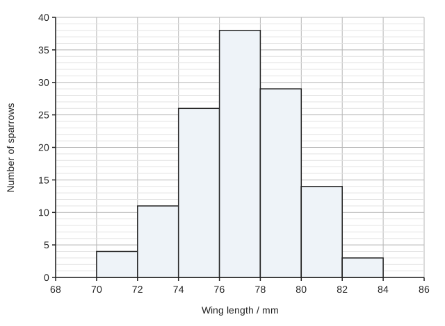
A histogram of number of sparrows (y-axis, 0 to 40) against wing length in mm (x-axis, 68 to 86). There are seven touching bars, each 2 mm wide: 70 to 72 mm, 4 sparrows; 72 to 74 mm, 11; 74 to 76 mm, 26; 76 to 78 mm, 38; 78 to 80 mm, 29; 80 to 82 mm, 14; 82 to 84 mm, 3.

Model answer

Sparrows with a wing length of 78 mm or more = 29 + 14 + 3 = 46
Percentage = 46 ÷ 125 × 100 = 36.8 = 37% (2 significant figures)

Wing length is a continuous variable. The classes follow on from each other with no gaps, so the bars of a histogram touch, whereas a bar chart has separate bars for separate categories.

None of the 125 sparrows measured had wings shorter than 70 mm, but this was only a sample. The frequencies fall gradually towards 70 mm, so a few sparrows in the whole population could have shorter wings and not have been caught.

Explanation

A histogram shows the frequency distribution of a continuous variable that has been grouped into classes, so the bars touch. Read each bar height carefully from the grid: the classes of 78 mm or more are 78-80, 80-82 and 82-84 mm, and the answer must be rounded to 2 significant figures. A sample shows the range of its own values, not of the whole population: rare extreme values are easily missed, especially where the frequencies tail off rather than stopping abruptly.

Mark scheme

1 mark
37 (%), from (29 + 14 + 3) ÷ 125 × 100 = 46 ÷ 125 × 100; a correct answer of 37 with no working scores this mark
Max 3. A correct answer of 37 (%) with no working scores this mark. Do not accept 36.8 (not given to 2 significant figures) or 67 (84 ÷ 125 × 100, the 76-78 mm class included).
1 mark
Wing length is a continuous variable / the data are continuous (grouped into classes with no gaps between them)
Accept "there are no gaps between the classes, so the bars touch". Ignore "there are a lot of data". Reject "wing length is categoric / discrete".
1 mark
Only a sample of 125 sparrows was measured, so rare sparrows with shorter wings may be present in the area but were not caught
Points 3 to 5: max 1. Ignore 'none of the 125 sparrows had wings shorter than 70 mm' on its own (it only restates the data).
1 mark
The numbers fall gradually towards 70 mm (only 4 sparrows in the 70-72 mm class), so a larger sample would be likely to include a few sparrows with shorter wings / the distribution may continue below 70 mm
1 mark
The sparrows caught may not be a random sample of those in the area (e.g. some birds are less likely to be caught), so birds with shorter wings may have been missed

Question 2

3 marks

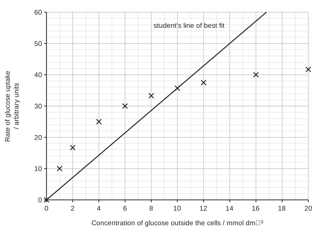
Yeast cells take up glucose by facilitated diffusion. A student measured the rate of glucose uptake by yeast cells at different concentrations of glucose outside the cells. The figure shows her results and the straight line of best fit that she drew through the origin.

Evaluate her straight line of best fit through the origin. Use your knowledge of facilitated diffusion in your answer.

A graph of rate of glucose uptake in arbitrary units (y-axis, 0 to 60) against concentration of glucose outside the cells in mmol dm⁻³ (x-axis, 0 to 20). Ten points are plotted as crosses: (0, 0), (1, 10), (2, 16.7), (4, 25), (6, 30), (8, 33.3), (10, 35.7), (12, 37.5), (16, 40) and (20, 41.7). A straight line labelled "student's line of best fit" runs from the origin through the point at 10 mmol dm⁻³ to the top of the graph at about 17 mmol dm⁻³.

Model answer

Drawing the line through the origin is justified, because with no glucose outside the cells there can be no uptake. However, a straight line is not appropriate: the points at low concentrations lie above the line and those at high concentrations lie below it, so the points form a curve that levels off. The rate levels off because the number of carrier proteins in the cell-surface membrane is limited; at high concentrations of glucose they are all in use. She should have drawn a smooth curve of best fit through the origin.

Explanation

When choosing a line of best fit, decide whether the data follow a straight line or a curve, and whether (0, 0) is a real point. Facilitated diffusion through carrier proteins reaches a maximum rate when all the carriers are occupied, so the curve levels off; with simple diffusion the rate would keep rising in proportion to the concentration gradient.

Mark scheme

1 mark
Drawing the line through the origin is correct because there is no uptake when there is no glucose outside the cells
Max 3, with at most 1 mark from point 1 (for the line) and at most 2 marks from points 2 to 4 (against it). Accept "(0, 0) is a real point".
1 mark
The points do not lie on a straight line: those at low concentrations are above the line and those at high concentrations are below it / the points form a curve that levels off
Accept "the relationship is not linear / not proportional".
1 mark
A (smooth) curve of best fit should have been drawn
1 mark
The rate levels off because the number of carrier proteins is limited / the carrier (or channel) proteins become saturated / are all in use at high glucose concentrations
Reject "ATP runs out" (facilitated diffusion does not use ATP from respiration). Accept "transport proteins" for carrier proteins.

Question 3

4 marks

Scientists carried out four investigations, A to D.

A The mean number of eggs laid per day by female blowflies kept at 15, 20, 25, 30 and 35 °C.
B The mean concentration of protein in the seeds of five varieties of soya bean.
C The masses of 200 hen's eggs from one farm, sorted into classes of 50.0-54.9 g, 55.0-59.9 g and so on.
D The body length of each of 40 female three-spined sticklebacks and the number of eggs that each female produced.

Name the most suitable type of graph for presenting the results of each investigation.

Model answer

A: line graph
B: bar chart
C: histogram
D: scatter graph

Explanation

A line graph is used when the independent variable is continuous and set by the investigator, such as temperature. A bar chart, with separate bars, is used when the independent variable is categoric, such as variety. A histogram shows how often values of one continuous variable fall into each class, so its bars touch. A scatter graph shows whether two measured variables are correlated, and its points are not joined. A common error is to use a bar chart for grouped continuous data such as masses.

Mark scheme

1 mark
A: line graph
1 mark for each investigation. If more than one type of graph is given for an investigation, do not award the mark for that investigation. A: accept a line graph with the points joined by straight lines or by a curve of best fit. Reject bar chart.
1 mark
B: bar chart
Accept bar chart with separate bars. Reject histogram and line graph.
1 mark
C: histogram
Accept frequency histogram. Reject bar chart (the masses are continuous data grouped into classes).
1 mark
D: scatter graph / scattergram / scatter diagram
Accept scatter graph with a line of best fit. Reject line graph.

Question 4

5 marks

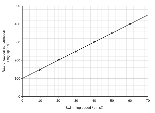
Scientists measured the rate of oxygen consumption of Atlantic salmon swimming at different speeds in a water channel. The figure shows the mean results and a line of best fit.

The line of best fit can be written in the form y = mx + c.

Use the figure to find the values of m and c. Suggest what the value of c represents.

Use your values to predict the rate of oxygen consumption at a swimming speed of 90 cm s⁻¹. Evaluate this prediction.

A graph of rate of oxygen consumption in mg kg⁻¹ h⁻¹ (y-axis, 0 to 500, grid lines every 20) against swimming speed in cm s⁻¹ (x-axis, 0 to 70, grid lines every 2). Six mean values are plotted as crosses at 10, 20, 30, 40, 50 and 60 cm s⁻¹, rising steadily. A straight line of best fit runs from the y-axis to a speed of 70 cm s⁻¹; its position can be read from the grid.

Model answer

From the line: at x = 0, y = 100; at x = 70, y = 450
m = (450 - 100) ÷ 70 = 5 and c = 100, so y = 5x + 100

c is the rate of oxygen consumption when the salmon is not swimming: its resting metabolic rate.

At 90 cm s⁻¹: y = 5 × 90 + 100 = 550 mg kg⁻¹ h⁻¹

This prediction may not be valid, because 90 cm s⁻¹ is outside the range of speeds measured (it is an extrapolation). At higher speeds the relationship may not be linear, for example if the fish reaches its maximum rate of oxygen uptake and respires anaerobically.

Explanation

In y = mx + c, m is the gradient (change in y ÷ change in x) and c is the intercept on the y-axis. Here the intercept has a biological meaning: the oxygen used when the swimming speed is zero. Predictions within the range of the data (interpolation) are more reliable than predictions beyond it (extrapolation), because the relationship may change outside the range measured.

Mark scheme

1 mark
m = 5 (accept 4.8 to 5.2)
A correct value of m with no working scores this mark; m is the gradient, e.g. (450 - 100) ÷ 70 or (400 - 150) ÷ (60 - 10). Ignore units. Accept m found from two plotted points if the value is in the range.
1 mark
c = 100 (accept 95 to 105)
c is the intercept on the y-axis (the value of y when x = 0). A correct value with no working scores this mark.
1 mark
(c is) the rate of oxygen consumption at rest / when the fish is not swimming / the resting (standard) metabolic rate
Accept "oxygen used for processes other than swimming, e.g. maintaining the body". Ignore "the starting value".
1 mark
550 (mg kg⁻¹ h⁻¹)
ECF: accept 90 × m + c using the values of m and c given in the answer. A correct value with no working scores this mark.
1 mark
The prediction may not be valid because 90 cm s⁻¹ is outside the range of the data (extrapolation) OR the relationship may not stay linear at higher speeds, e.g. the fish may reach its maximum rate of oxygen uptake / respire anaerobically / be unable to swim that fast
Credit one evaluative point. Ignore "the fish might be different sizes" or "the scientists should repeat it".

Ready to try the rest? Every answer you write is marked against the mark scheme, so you can see exactly where the marks are.

Study Helper Hints first, answers after you try

Stuck on this one? Ask for a hint and I’ll point you in the right direction, without giving the answer away. Once you’ve checked your answer, I’ll show you how the marks are awarded.