Level:
Correct: 0
Incorrect: 0
Marks: 0/0
Exam Practice
Course:
Topics:
AQA GCSE Economics (Paper 1) Smart practice A mixed round aimed at your weak spots
Unit 1
Economic foundations
Economic activity
Economic activity
The factors of production
Unit 2
Resource allocation
Markets and allocation of resources
Markets and the allocation of resources
Economic sectors
Economic sectors
Specialisation, division of labour, and exchange
Specialisation, division of labour and exchange
Unit 3
How prices are determined
Demand for goods and services
Supply for goods and services
Supply of goods and services
Equilibrium price
Equilibrium price
Intermarket relationships
Price elasticity of demand
Price elasticity of supply
Unit 4
Production, costs, revenue and profit
The importance of cost, revenue and profit for producers
Cost, revenue and profit for producers
Production and productivity
Economies of scale
Economies of scale
Unit 5
Competitive and concentrated markets
The importance of market structures on producers and consumers
Market structures
Competitive markets
Competitive markets
The labour market
The labour market
Unit 6
Market failure
Avg
score:
–
Topics
done:
0/21

Price elasticity of supply

Practise 15 exam-style questions on Price elasticity of supply for AQA GCSE Economics (Paper 1). Write your answer as you would in the exam and get it marked in seconds against the mark scheme, point by point, with the Study Helper on hand if you get stuck.

  • 15 questions
  • 1–15 marks each
  • Instant marking
  • No sign-up needed
15 questions, marked as you go

Sample questions with model answers

Here are 4 of the questions in this topic, each with a model answer, an explanation of why it earns the marks and the mark scheme an examiner would use.

Question 1

1 mark

The price of a product rises from £20 to £23. The quantity supplied rises from 5,000 to 6,200 units a week.

What is the price elasticity of supply?

Choose your answer.

  • A 0.625
  • B 1.48
  • C 1.6
  • D -1.6

Model answer

C 1.6

Explanation

% change in quantity supplied = (6,200 - 5,000) ÷ 5,000 × 100 = 24%; % change in price = (23 - 20) ÷ 20 × 100 = 15%; PES = 24 ÷ 15 = 1.6, so supply is price elastic. 0.625 is the formula upside down, 1.48 uses the new values as the base, and -1.6 has the wrong sign: PES is positive because price and quantity supplied move in the same direction.

Mark scheme
  1. 1 mark

    C / 1.6

    Accept the letter or the option text. If more than one option is given, 0 marks.

Question 2

2 marks

A craft workshop makes wooden toys. When the price of its toys rises from £16 to £20, the number it supplies each month rises from 300 to 345.

Calculate the price elasticity of supply of the toys.

Model answer

% change in quantity supplied = (345 - 300) ÷ 300 × 100 = 15%
% change in price = (20 - 16) ÷ 16 × 100 = 25%
PES = 15 ÷ 25 = 0.6

Explanation

PES = % change in quantity supplied ÷ % change in price, with each change worked out as a percentage of the original value. The answer, 0.6, is below 1, so supply is price inelastic: hand-made toys take time to make, so output cannot rise as fast as the price. The usual errors are turning the formula upside down and using the new values as the base.

Mark scheme
  1. 1 mark

    Correct method, e.g. % change in quantity supplied = (345 - 300) ÷ 300 × 100 = 15% and % change in price = (20 - 16) ÷ 16 × 100 = 25%, or PES = 15 ÷ 25; or a correct final answer of 0.6 with no working

    An answer of 0.6 with no working scores 2 marks. Award this mark for both percentage changes correct (15% and 25%) even if the final answer is wrong. The formula upside down (25 ÷ 15 = 1.67) scores 1 only if both percentage changes are shown correctly. Using the new values as the base (13.0% ÷ 20% = 0.65) scores 0. Dividing the absolute changes (45 ÷ £4 = 11.25) scores 0.

  2. 1 mark

    0.6 (accept 0.60 / +0.6 / 3/5)

    -0.6 scores 1 mark in total: PES for an upward-sloping supply curve is positive. Ignore a correct extra comment such as 'supply is price inelastic'.

Question 3

3 marks

The price paid to recycling firms for a tonne of recycled plastic rises from £340 to £410. The quantity of recycled plastic supplied each month rises from 18,500 tonnes to 20,200 tonnes.

Calculate the price elasticity of supply of recycled plastic. Give your answer to two decimal places.

Model answer

% change in quantity supplied = (20,200 - 18,500) ÷ 18,500 × 100 = 9.19%
% change in price = (410 - 340) ÷ 340 × 100 = 20.59%
PES = 9.19 ÷ 20.59 = 0.446... = 0.45 (to 2 decimal places)

Explanation

Work out both percentage changes from the original values (18,500 tonnes and £340), then divide the change in quantity supplied by the change in price. PES is 0.45, below 1, so supply is price inelastic: recycling firms cannot quickly collect and process much more plastic. Marks are lost for rounding wrongly or for dividing the price change by the quantity change.

Mark scheme
  1. 1 mark

    A correct percentage change: quantity supplied (20,200 - 18,500) ÷ 18,500 × 100 = 9.19% or price (410 - 340) ÷ 340 × 100 = 20.59%; or a correct final answer of 0.45 with no working

    An answer of 0.45 with no working scores 3 marks. Answer not to two decimal places but otherwise correct (e.g. 0.446 or 0.4): 2 marks. The formula upside down (20.59 ÷ 9.19 = 2.24) scores 1 if a correct percentage change is shown. Using the new values as the base (8.42% ÷ 17.07% = 0.49) scores 0. Dividing the absolute changes (1,700 ÷ £70) scores 0. Accept 9.2% and 20.6% for the percentage changes.

  2. 1 mark

    Correct method: % change in quantity supplied ÷ % change in price with both percentages correct, e.g. 9.19 ÷ 20.59 (implied by a correct final answer)

    Percentage changes rounded to whole numbers (9 ÷ 21 = 0.43) score 2: correct method, but too inaccurate for the final mark.

  3. 1 mark

    0.45

    The unrounded value is 0.4463..., so supply is price inelastic. -0.45 scores 2 at most. Ignore a correct comment about elasticity.

Question 4

9 marks

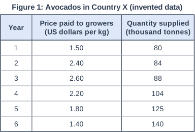
Country X is a major grower of avocados. Avocado trees take about four years after planting to produce fruit. In Year 2, demand for avocados from Country X rose sharply as they became more popular in Europe, and many growers planted new trees. Most growers are small family farms, and planting and watering new trees is expensive. Figure 1 shows the price paid to growers and the quantity of avocados supplied from Year 1 to Year 6 (invented data).

Using Figure 1, assess whether the increase in demand for avocados has benefited growers in Country X.

Figure 1: Avocados in Country X (invented data). Table with columns "Year", "Price paid to growers (US dollars per kg)", "Quantity supplied (thousand tonnes)". Year: 1; Price paid to growers (US dollars per kg): 1.50; Quantity supplied (thousand tonnes): 80 | Year: 2; Price paid to growers (US dollars per kg): 2.40; Quantity supplied (thousand tonnes): 84 | Year: 3; Price paid to growers (US dollars per kg): 2.60; Quantity supplied (thousand tonnes): 88 | Year: 4; Price paid to growers (US dollars per kg): 2.20; Quantity supplied (thousand tonnes): 104 | Year: 5; Price paid to growers (US dollars per kg): 1.80; Quantity supplied (thousand tonnes): 125 | Year: 6; Price paid to growers (US dollars per kg): 1.40; Quantity supplied (thousand tonnes): 140.

Model answer

In the short run the increase in demand clearly benefited existing growers. Because avocado trees take about four years to produce fruit, supply was very price inelastic: between Year 1 and Year 2 the price rose by 60%, from 1.50 to 2.40 US dollars per kg, but the quantity supplied rose by only 5%, from 80 to 84 thousand tonnes, giving a PES of about 0.08. As a result growers' total revenue rose from about 120 million US dollars (80,000 tonnes × 1.50 per kg) to about 201.6 million in Year 2 and 228.8 million in Year 3. Growers who already had trees gained most, because their costs hardly changed while the price of what they sold rose sharply, so their profits rose. The higher price also acted as a signal and an incentive to expand production.

However, the benefits did not last. Many growers planted new trees, which cost money for land, water and labour but earned nothing for about four years. When the new trees began to produce fruit from Year 4, supply shifted to the right: quantity rose to 140 thousand tonnes in Year 6 while the price fell to 1.40 US dollars per kg, below its Year 1 level. Total revenue fell to about 196 million US dollars in Year 6. That is still higher than in Year 1, but it is now shared among more growers, and with more trees to look after, total costs are much higher. So profit per grower, especially for those who planted late and borrowed to do so, may be lower than before demand rose.

Overall, the increase in demand benefited growers in Country X in the short run, because inelastic supply meant the extra demand raised prices rather than quantity. In the long run the benefit is much less clear, because the growers' own response increased supply and pushed the price down. Whether growers have gained overall depends on when they planted, on their costs (especially water and loans) and on whether demand in Europe keeps rising; if it does, the lower price in Year 6 may only be temporary.

Explanation

Strong answers use Figure 1 to show that supply was price inelastic at first (a 60% price rise with a 5% rise in quantity) and calculate revenue, then explain how the lagged supply response pushed the price down later. Level 3 needs a judgement that distinguishes the short run from the long run and says what the answer depends on. Answers that use no data, or consider only the benefits, cannot score more than 6.

Mark scheme
  1. 9 marks

    Levels of response (9 marks).
    Level 3 (7-9 marks): A fully justified conclusion with sustained evaluation, which is coherent and relevant, with judgements supported by evidence. A full analysis of the economic evidence, a well-developed and logical chain of reasoning. Comprehensive application of knowledge and understanding of pertinent concepts/issues relevant to the context; specialist language used throughout.
    Level 2 (4-6 marks): A partially justified conclusion with an evaluation, which is mostly coherent and relevant; judgements may not be fully supported by evidence. An incomplete analysis of the economic evidence; starts to develop a chain of reasoning. Good application of knowledge and understanding of concepts/issues mostly relevant to the context; specialist language used mostly appropriately.
    Level 1 (1-3 marks): A basic conclusion or assertion may be present based on evaluative judgements supported by little or no evidence. Analysis of discrete points of the economic evidence with no chain of reasoning attempted. Basic application of knowledge and understanding of concepts/issues with limited relevance to the context; may use non-specialist language.
    0 marks: Nothing written worthy of credit.

    Max 6 if the answer considers only one side or gives no judgement. Max 6 if the answer makes no use of the figure/data given. Indicative content (not exhaustive; credit other valid points). Benefits: in the short run supply was very price inelastic (trees take years to bear fruit): between Year 1 and Year 2 the price rose 60% (1.50 to 2.40 US dollars per kg) while quantity supplied rose only 5% (80 to 84 thousand tonnes), PES about 0.08. So growers' total revenue rose sharply, from about 120 million US dollars in Year 1 to about 201.6 million in Year 2 and 228.8 million in Year 3. Existing growers gained most, as their costs barely changed. High prices gave an incentive to plant and expand (higher prices imply higher profits). Total revenue in Year 6 (196 million) is still well above Year 1, and output is 75% higher. Costs: growers could not take full advantage at first because supply could not respond. New trees cost money to plant and water and earn nothing for about four years. From Year 4 the new trees produced fruit, supply shifted to the right and the price fell, to 1.40 US dollars per kg in Year 6, below its Year 1 level; revenue per kg is lower, revenue is shared among more growers, and total costs are higher with more trees, so profits per grower may be lower than before. Growers who planted late may not cover their costs. Note: after Year 3 price fell while quantity rose, so these years show supply shifting, not a movement along the original supply curve. Use of data: price and quantity changes, PES for Years 1-2, total revenue by year. Overall: growers benefited strongly in the short run, especially existing ones; long-run benefits are smaller and uncertain. The judgement may depend on the time period, growers' costs, whether demand keeps rising, and when each grower planted.

Ready to try the rest? Every answer you write is marked against the mark scheme, so you can see exactly where the marks are.

Study Helper Hints first, answers after you try

Stuck on this one? Ask for a hint and I’ll point you in the right direction, without giving the answer away. Once you’ve checked your answer, I’ll show you how the marks are awarded.