Histograms, box plots and cumulative frequency - Edexcel A-Level Maths (Paper 3) Exam Questions

Practise 19 exam-style questions on Histograms, box plots and cumulative frequency for Edexcel A-Level Maths (Paper 3). Write your answer as you would in the exam and get it marked in seconds against the mark scheme, point by point, with the Study Helper on hand if you get stuck.

19 questions
3–9 marks each
Instant marking
No sign-up needed

19 questions, marked as you go

Sample questions with model answers

Here are 4 of the questions in this topic, each with a model answer, an explanation of why it earns the marks and the mark scheme an examiner would use.

Question 1

4 marks

The histogram shows the lengths, \(l\) cm, of the runner beans picked from a school's vegetable garden in one week. The frequency density axis has no scale.

26 of the beans have lengths between 18 cm and 20 cm.

Estimate the number of beans with lengths greater than 22 cm.

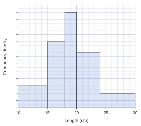
Histogram drawn on a grid of small squares. The horizontal axis is "Length (cm)", from 10 to 30, numbered every 5, with 5 small squares between numbered values (each small square is 1). The vertical axis is "Frequency density"; it has tick marks every 2 small squares but no numbers. The bars touch, with no gaps between them. Bars: from 10 to 15 (5 small squares wide), 6 small squares tall; from 15 to 18 (3 small squares wide), 18 small squares tall; from 18 to 20 (2 small squares wide), 26 small squares tall; from 20 to 24 (4 small squares wide), 15 small squares tall; from 24 to 30 (6 small squares wide), 4 small squares tall.

Model answer

The 18-20 cm bar is 2 small squares wide and 26 small squares tall, so its area is 52 small squares, which represents 26 beans. So 1 small square of area represents 0.5 beans.
(Equivalently, its frequency density is \(\dfrac{26}{2} = 13\), so each small square up the axis is 0.5.)
22 cm to 24 cm: the 20-24 cm bar is 15 small squares tall, so this part has area \(2 \times 15 = 30\) small squares: 15 beans.
24 cm to 30 cm: the bar is 4 small squares tall, so its area is \(6 \times 4 = 24\) small squares: 12 beans.
Estimate \(= 15 + 12 = 27\) beans

Explanation

In a histogram the area of each bar represents the frequency, so the bar whose frequency is given fixes the scale: 52 small squares of area represent 26 beans. Only the part of the 20-24 cm bar above 22 cm is used, assuming the beans are spread evenly through that class, which gives 15 beans, plus 12 from the last bar. A common error is to use the heights of the bars as frequencies.

Mark scheme

1 mark
M1 Uses the 18-20 cm bar to find the scale: its frequency density is \(26 \div 2 = 13\), so each small square up the axis is 0.5; or its area of \(2 \times 26 = 52\) small squares represents 26 beans, so 1 small square of area represents 0.5 beans; or a correct final answer of 27 with no working
An answer of 27 with no working scores 4 marks.
1 mark
M1 (dM1) Finds the number of beans for at least one of: the part of the 20-24 cm bar from 22 cm to 24 cm; the 24-30 cm bar
Depends on the M mark just before it. Using the whole of the 20-24 cm bar (30 beans) instead of the part from 22 to 24 cm is M0.
1 mark
A1 15 beans from 22 cm to 24 cm and 12 beans from 24 cm to 30 cm
Both needed.
1 mark
A1 27 beans
Depends on both M marks. cao.

Question 2

4 marks

The 19 members of a fitness class each did as many push-ups as they could in one minute. For their results, the lowest value was 12, the lower quartile 20, the median 27, the upper quartile 33 and the highest value 45. There were no outliers.

Two new members join the class. They do 8 and 50 push-ups.

An outlier is a value that is more than \(1.5 \times\) (interquartile range) above the upper quartile or below the lower quartile. You may assume that the quartiles are not changed by the two new values.

State, with a reason, the effect of the two new values on the median.

Determine whether either new value is an outlier, and describe how the box plot for all 21 members differs from the box plot for the original 19 members.

Model answer

The median is unchanged at 27: one new value (8) is below 27 and the other (50) is above it, so the middle value of the 21 results is the same as the middle value of the original 19.
Interquartile range \(= 33 - 20 = 13\)
Lower limit \(= 20 - 1.5 \times 13 = 0.5\); upper limit \(= 33 + 1.5 \times 13 = 52.5\)
\(8 > 0.5\) and \(50 < 52.5\), so neither new value is an outlier.
The box (lower quartile, median, upper quartile) stays the same, but the whiskers now reach 8 and 50 instead of 12 and 45, so the range increases from 33 to 42.

Explanation

Adding one value below the median and one above it moves the middle position along by one, so the median value does not change. The outlier test uses the limits 1.5 interquartile ranges beyond the quartiles, and both new values lie inside them, so they become the new ends of the whiskers. A box plot changes only where its five summary values change.

Mark scheme

1 mark
B1 The median is unchanged (27): one new value is below it and one is above it, so the middle (11th) of the 21 values is the same as the middle (10th) of the original 19. Answers with no working or reasons score 1 mark (see comments).
An answer of "median unchanged; neither value is an outlier; the whiskers now end at 8 and 50" with no working scores 1 mark (the final B1, for the whiskers): the median mark needs a reason, and the limits must be shown for the M1 A1. "The median changes" scores B0.
1 mark
M1 Finds the limits: \(20 - 1.5 \times 13 = 0.5\) and \(33 + 1.5 \times 13 = 52.5\)
Both limits needed.
1 mark
A1 Neither value is an outlier, since \(0.5 < 8\) and \(50 < 52.5\)
1 mark
B1 The box (quartiles and median) is unchanged, but the whiskers now extend to 8 and 50 (so the range increases from 33 to 42)
Needs both whisker ends (or the idea that both whiskers get longer, to 8 and 50). ft their outlier decision: if they think a value is an outlier, the whisker on that side stays at the old end and the value is plotted as a cross.

Question 3

5 marks

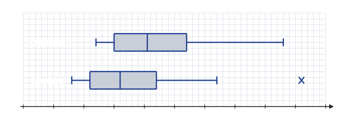
The box plots in the diagram summarise the Daily Maximum Gust, in knots, at Camborne and at Leuchars in October 2015, taken from the large data set. The Leuchars box plot uses all 31 days of October, but the Camborne box plot uses only 30 days. An outlier, shown with a cross, is a value that is more than \(1.5 \times\) (interquartile range) above the upper quartile or below the lower quartile.

Suggest a reason why the Camborne box plot uses only 30 days.

Compare the Daily Maximum Gusts at the two stations in October 2015.

The outlier on the Leuchars box plot is the gust on 22/10/2015. On that day the Daily Mean Windspeed at Leuchars was 22 kn, with a Beaufort conversion of Strong. A student says that this outlier should be removed before the two stations are compared. Comment on the student's suggestion.

Two box plots, one above the other, drawn above a horizontal scale "Daily Maximum Gust (kn)" from 0 to 50, numbered every 5, on a grid of small squares (each small square is 1). The top box plot is labelled "Camborne" and the bottom one "Leuchars". For each box plot, the ends of the whiskers, the quartiles (sides of the box) and the median (line inside the box) can be read from the scale. A cross (outlier) is drawn to the right of the right whisker of the Leuchars box plot; its value can be read from the scale.

Model answer

One day's Daily Maximum Gust at Camborne in October 2015 is n/a (not available), so only 30 days could be used.
The median gust at Camborne (20.5 kn) is higher than at Leuchars (16 kn), so the gusts were generally stronger at Camborne.
The interquartile ranges are similar (\(27 - 15 = 12\) kn and \(22 - 11 = 11\) kn), but Leuchars has the larger range (38 kn against 31 kn) because of its outlier.
On 22/10/2015 the mean windspeed at Leuchars was 22 kn, Beaufort Strong, so a gust of 46 kn is consistent with the weather that day and is likely to be genuine. It should not be removed: it is a real, if extreme, observation.

Explanation

In the large data set n/a marks data that are not available, and at the UK stations in 2015 the only missing values are for Camborne on 07/10/2015. Box plots are compared using the medians and a measure of spread, interpreted in context. An outlier should only be removed if there is evidence that it is an error; here the strong mean windspeed that day suggests the gust is genuine.

Mark scheme

1 mark
B1 The value for one day is missing: the Daily Maximum Gust at Camborne is n/a (not available) for one day in October 2015
Accept "missing data" or "n/a". (It is 07/10/2015; the date is not needed.) Do not accept "tr" or "October has 30 days".
1 mark
B1 Camborne has the higher median (20.5 kn against 16 kn), so the gusts were generally stronger at Camborne
Must compare medians and interpret in context (stronger or higher gusts).
1 mark
B1 A comparison of spread: the interquartile ranges are similar (12 kn at Camborne, 11 kn at Leuchars), but Leuchars has the greater range (38 kn against 31 kn) because of its outlier
Accept either a comparison of the interquartile ranges or of the ranges, with values or a correct statement.
1 mark
B1 The gust is consistent with the strong winds that day (a mean speed of 22 kn, Beaufort Strong), so it is likely to be a genuine value, not an error
Must use the windspeed or Beaufort information.
1 mark
B1 So it should not be removed: it is real data about the weather at Leuchars, even though it is extreme
Needs a conclusion that the value should be kept, with a reason (genuine data, not an error).

Question 4

6 marks

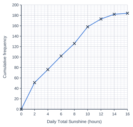
The cumulative frequency polygon shows the Daily Total Sunshine, \(x\) hours, at Hurn for the 184 days of 2015 in the large data set.

Use the graph to estimate the median and the interquartile range of the Daily Total Sunshine.

The median of the 184 values in the large data set is 5.3 hours. Give a reason why your estimate of the median is different.

Use the graph to find the number of days on which there were more than 10 hours of sunshine.

A student uses this to say that, at Hurn, about 14% of all the days in a year have more than 10 hours of sunshine. Explain why this is not a sensible conclusion.

Cumulative frequency graph on a grid of small squares. The horizontal axis is "Daily Total Sunshine (hours)", from 0 to 16, numbered every 2, with 4 small squares between numbered values (each small square is 0.5). The vertical axis is "Cumulative frequency", from 0 to 200, numbered every 20, with 5 small squares between numbered values (each small square is 4). Straight lines join (0, 0), (2, 51), (4, 76), (6, 102), (8, 126), (10, 158), (12, 173), (14, 182) and (16, 184) (each point is marked with a cross).

Model answer

Median: reading across from \(\dfrac{184}{2} = 92\) gives about 5.2 hours.
Quartiles: reading from 46 gives \(Q_1 \approx 1.8\) hours; reading from 138 gives \(Q_3 \approx 8.75\) hours.
Interquartile range \(\approx 8.75 - 1.8 = 6.95\) hours
The graph is drawn from grouped data and assumes the values are spread evenly within each class, so the median read from it is only an estimate of the true median, 5.3 hours.
At 10 hours the cumulative frequency is 158, so \(184 - 158 = 26\) days had more than 10 hours of sunshine.
The data cover only May to October, when the days are long. In November to April the days are much shorter, so far fewer days would have more than 10 hours of sunshine; 14% cannot be applied to the whole year.

Explanation

Readings from a cumulative frequency graph use \(\dfrac{n}{2}\), \(\dfrac{n}{4}\) and \(\dfrac{3n}{4}\), here 92, 46 and 138. Because the graph is built from grouped data, values read from it are estimates. The large data set has only May to October, so conclusions about a whole year, especially about sunshine, which depends on day length, are not valid.

Mark scheme

1 mark
B1 Median 5.2 hours (read at a cumulative frequency of 92; accept 5.0 to 5.5). Readings of the interquartile range and the number of days with no working score their marks.
An answer of 5.2, 6.95 and 26 with no working scores 4 marks: the values can be read from the graph; the two explanations are marked separately.
1 mark
M1 Reads the quartiles at cumulative frequencies 46 and 138 (\(Q_1 = 1.8\), \(Q_3 = 8.75\)) and subtracts
Accept \(Q_1\) from 1.6 to 2.0 and \(Q_3\) from 8.5 to 9.0.
1 mark
A1 Interquartile range 6.95 hours (accept 6.5 to 7.4)
1 mark
B1 The data are grouped, and the polygon assumes that the values are spread evenly within each class (straight lines between the points), so the median read from it is only an estimate
Accept "the exact values are not shown on the graph" or "the graph uses grouped data".
1 mark
B1 26 days (\(184 - 158\))
cao: the point at 10 hours is plotted.
1 mark
B1 The large data set covers only May to October, when the days are longest; in the winter months the days are much shorter, so the proportion for the whole year would be much smaller (and cannot be found from these data)
Must refer to the data covering only May to October (or summer months). Do not accept "184 days is too small a sample" on its own.

Ready to try the rest? Every answer you write is marked against the mark scheme, so you can see exactly where the marks are.

Study Helper Hints first, answers after you try

Stuck on this one? Ask for a hint and I’ll point you in the right direction, without giving the answer away. Once you’ve checked your answer, I’ll show you how the marks are awarded.